Cosmic-web formation: the Zel’dovich approximation

Zel’dovich (1970, “Gravitational instability: An approximate theory for large density perturbations”) showed that, to leading order, a fluid element of dark matter simply free-streams away from its initial (“Lagrangian”) position \(\mathbf{q}\) in a fixed direction set by the gradient of a displacement potential \(\Phi(\mathbf{q})\):

\[\mathbf{x}(\mathbf{q}, D) = \mathbf{q} - D\,\nabla\Phi(\mathbf{q}),\]

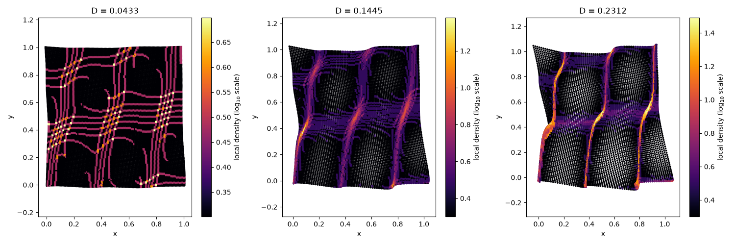
where \(D\) is the linear growth factor of density perturbations (\(D=0\) at the initial, unperturbed time, growing monotonically thereafter – in a flat, matter-dominated background, \(D\) is simply proportional to the scale factor \(a(t)\propto t^{2/3}\)). This example builds \(\Phi\) as a sum of a handful of random plane waves – a cheap stand-in for a realistic Gaussian random field – lays a regular grid of tracer particles over the Lagrangian coordinate \(\mathbf{q}\), and watches that grid warp into the cosmic web as \(D\) grows: first a gentle ripple, then sharp filaments and sheets (“pancakes”) as fluid elements pile up along their fastest-contracting direction, and finally a web of dense nodes where filaments cross.

The very first caustic (formally infinite density) anywhere in the field forms at

\[D_{\rm collapse} = \frac{1}{\max_{\mathbf{q}}\lambda_{\max}(\mathbf{q})},\]

where \(\lambda_{\max}(\mathbf{q})\) is the largest eigenvalue of the Hessian of \(\Phi\) at \(\mathbf{q}\) (physicskit.astro.cosmic_web.first_caustic_time()); this example sweeps \(D\) from 0 up through and somewhat past that value.

import matplotlib.pyplot as plt
import numpy as np

from physicskit.astro.cosmic_web import (
    first_caustic_time,
    lagrangian_grid,
    random_displacement_potential,
    zeldovich_hessian_eigenvalues,
    zeldovich_position,
)
from physicskit.astro.visualizers import animate_zeldovich_collapse, plot_zeldovich_snapshot

Build the displacement potential and the Lagrangian grid

A modest 8-mode random potential, with wavenumbers spanning about half a decade so structure forms across a controllable range of scales, laid over a 120x120 grid of tracer particles – dense enough to resolve filaments clearly while still animating in a few seconds.

box_size = 1.0
n_side = 120

k_vectors, amplitudes, phases = random_displacement_potential(
    n_modes=8,
    k_min=2 * np.pi / box_size,
    k_max=6 * np.pi / box_size,
    amplitude_scale=0.02,
    seed=7,
)
q = lagrangian_grid(n_side, box_size)

D_collapse = first_caustic_time(q, k_vectors, amplitudes, phases)
print(f"Analytic first-caustic growth factor (from the sampled grid): D_collapse = {D_collapse:.5f}")

Analytic first-caustic growth factor (from the sampled grid): D_collapse = 0.14448

Snapshots: uniform grid -> pancakes -> a web of nodes

Three snapshots at increasing growth factor: well before collapse (still nearly uniform, just gently rippled), right around the first caustic (sharp filaments/pancakes appear), and somewhat past it (the pancakes have crossed into a web with dense nodes at the intersections).

snapshot_D = [0.3 * D_collapse, 1.0 * D_collapse, 1.6 * D_collapse]
fig, axes = plt.subplots(1, 3, figsize=(15, 5))
for ax, D in zip(axes, snapshot_D):
    plot_zeldovich_snapshot(q, D, k_vectors, amplitudes, phases, ax=ax, s=3)
plt.tight_layout()

A collapse-time map baked into the Lagrangian grid

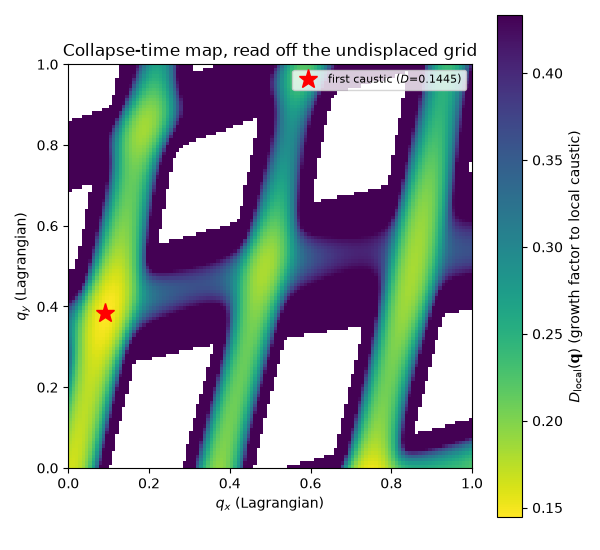
The pancake network in the three snapshots above is not a surprise that only appears once the field is displaced: it is already fully encoded, before any displacement is applied, in the local Hessian eigenvalues of the potential (zeldovich_hessian_eigenvalues()), the same per-point quantity first_caustic_time() maximizes over. Inverting the larger eigenvalue at each Lagrangian grid point gives a local “time-to-caustic” \(D_{\rm local}(\mathbf{q}) = 1/\lambda_{\max}(\mathbf{q})\): a 2D map, over the undisplaced grid, of how soon each fluid element collapses along its fastest-contracting direction. Its ridge lines (small \(D_{\rm local}\)) are the skeleton of the pancake network seen forming above, and its global minimum is exactly \(D_{\rm collapse}\) from the analytic formula. Blank (white) patches are points with \(\lambda_{\max}\le 0\) – expanding in every direction, so \(D_{\rm local}=\infty\): these become the voids of the cosmic web, never a caustic.

eigs = zeldovich_hessian_eigenvalues(q, k_vectors, amplitudes, phases)
lambda_max = eigs[:, 1]
with np.errstate(divide="ignore"):
    D_local = np.where(lambda_max > 0, 1.0 / lambda_max, np.inf)
D_local_grid = D_local.reshape(n_side, n_side).T  # rows: q_y, cols: q_x

i_min = np.argmin(D_local)
q_first_collapse = q[i_min]

fig_map, ax_map = plt.subplots(figsize=(6, 5.5))
im = ax_map.imshow(
    D_local_grid,
    origin="lower",
    extent=[0, box_size, 0, box_size],
    cmap="viridis_r",
    vmax=3 * D_collapse,
)
fig_map.colorbar(im, ax=ax_map, label=r"$D_{\rm local}(\mathbf{q})$ (growth factor to local caustic)")
ax_map.plot(*q_first_collapse, "r*", ms=14, label=f"first caustic ($D$={D_local[i_min]:.4f})")
ax_map.set_xlabel(r"$q_x$ (Lagrangian)")
ax_map.set_ylabel(r"$q_y$ (Lagrangian)")
ax_map.set_title("Collapse-time map, read off the undisplaced grid")
ax_map.legend(loc="upper right", fontsize=8)
ax_map.set_aspect("equal")
fig_map.tight_layout()
print(f"Collapse-time map: min(D_local) = {D_local[i_min]:.5f} vs analytic D_collapse = {D_collapse:.5f} (should match to grid resolution)")

Collapse-time map: min(D_local) = 0.14448 vs analytic D_collapse = 0.14448 (should match to grid resolution)

Animation: watching the grid collapse

Sweep D from 0 up to 1.6x the first-caustic time and animate the particles streaming from a perfectly regular grid into filaments, sheets, and nodes, colored by a local point-density proxy.

D_values = np.linspace(0.0, 1.6 * D_collapse, 60)
anim = animate_zeldovich_collapse(q, D_values, k_vectors, amplitudes, phases, interval=80, s=3)

# To save the animation to a file instead of (or in addition to) displaying
# it interactively, use e.g.::
#
#     anim.save("cosmic_web_collapse.gif", writer="pillow", fps=15)

plt.show()

Sanity check: numerically observed clumping versus the analytic prediction

Scan D finely and track the densest 2D-histogram bin at each step (the same local-density proxy used by the visualizers). The growth factor at which that peak density first crosses well above the uniform background level is the numerically observed onset of significant clumping – compare it to the analytic D_collapse computed above.

n_bins = max(20, int(np.sqrt(q.shape[0])))
uniform_count = q.shape[0] / n_bins**2
clump_threshold = 5.0 * uniform_count  # 5x the uniform-background bin count

D_scan = np.linspace(0.0, 2.0 * D_collapse, 400)
D_numeric_onset = None
for D in D_scan:
    x = zeldovich_position(q, D, k_vectors, amplitudes, phases)
    counts, _, _ = np.histogram2d(x[:, 0], x[:, 1], bins=n_bins)
    if counts.max() > clump_threshold:
        D_numeric_onset = D
        break

print(f"Analytic first-caustic growth factor:              D_collapse       = {D_collapse:.5f}")
if D_numeric_onset is not None:
    print(f"Numerically observed onset of significant clumping: D_numeric_onset = {D_numeric_onset:.5f}")
    print(f"Ratio D_numeric_onset / D_collapse = {D_numeric_onset / D_collapse:.3f}")
    print(
        "(expected to be somewhat below 1: a finite-count detection threshold on a "
        "finite grid necessarily fires before the continuum's true density divergence "
        "is reached, but should land in the same right ballpark as D_collapse)"
    )
else:
    print("No significant clumping detected in the scanned range.")

Analytic first-caustic growth factor:              D_collapse       = 0.14448
Numerically observed onset of significant clumping: D_numeric_onset = 0.10356
Ratio D_numeric_onset / D_collapse = 0.717
(expected to be somewhat below 1: a finite-count detection threshold on a finite grid necessarily fires before the continuum's true density divergence is reached, but should land in the same right ballpark as D_collapse)