Rotation curves, the NFW halo, and the dark-matter mass discrepancy

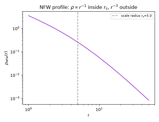
Three results form one chain. Oort (1932) and Zwicky (1933) applied the virial theorem to stellar and galaxy-cluster velocities and found implied masses far exceeding the visible matter. Rubin and Ford (1970), confirmed and extended through the 1970s by Roberts, Whitehurst, Bosma, and others, measured spiral-galaxy rotation curves that stayed flat far beyond the visible disk rather than falling off as Keplerian motion around a centrally concentrated mass predicts. Navarro, Frenk, and White (1996-1997) found that cosmological dark-matter halos collapse onto a single near-universal density profile,

\[\rho_{\rm NFW}(r) = \frac{\rho_s}{(r/r_s)(1+r/r_s)^2},\]

that reproduces exactly the flat curves observed. This example builds both a visible-matter-only rotation curve and an NFW halo’s rotation curve with circular_velocity(), compares them directly, and reproduces the historical virial-theorem logic that first suggested unseen mass was there at all.

import matplotlib.pyplot as plt
import numpy as np

from physicskit.astro.galactic_dynamics import (
    circular_velocity,
    nfw_density,
    nfw_enclosed_mass,
)
from physicskit.astro.visualizers import plot_rotation_curve

Visible matter alone: a Keplerian falloff

Beyond a galaxy’s visible disk, essentially all the visible mass is already enclosed, so a test star’s circular velocity should fall as \(v_c\propto1/\sqrt r\) – ordinary Newtonian motion around a fixed, centrally concentrated mass. This is exactly what Rubin and Ford expected to see, and did not.

M_visible = 50.0
r_values = np.linspace(1.0, 50.0, 300)
v_visible = circular_velocity(r_values, lambda r: np.full_like(r, M_visible))

An NFW halo: a flat rotation curve

rho_s, r_s = 1.0, 5.0
v_nfw = circular_velocity(r_values, lambda r: nfw_enclosed_mass(r, rho_s, r_s))

fig1, ax1 = plot_rotation_curve(r_values, v_nfw)
ax1.plot(r_values, v_visible, "--", color="firebrick", label="visible matter only (Keplerian)")
ax1.lines[0].set_label("NFW dark-matter halo (flat)")
ax1.set_title("Rubin-Ford: flat curves, not the Keplerian falloff visible matter predicts")
ax1.legend(fontsize=8)
fig1.tight_layout()

print(f"v_c at r=40 (visible matter only): {circular_velocity(40.0, lambda r: M_visible):.4f}  (still falling)")
print(f"v_c at r=40 (NFW halo):            {circular_velocity(40.0, lambda r: nfw_enclosed_mass(r, rho_s, r_s)):.4f}")
print(f"v_c at r=20 (NFW halo):            {circular_velocity(20.0, lambda r: nfw_enclosed_mass(r, rho_s, r_s)):.4f}  (nearly the same -- flat)")

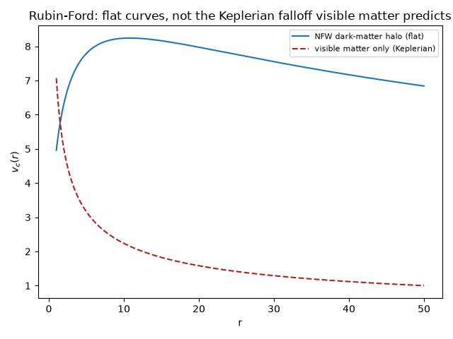
v_c at r=40 (visible matter only): 1.1180  (still falling)
v_c at r=40 (NFW halo):            7.1679
v_c at r=20 (NFW halo):            7.9733  (nearly the same -- flat)

Zwicky’s virial-mass estimate vs. the visible mass

Decades before the NFW profile existed to describe the halo, Zwicky inferred a cluster’s total mass purely from its members’ velocity dispersion and the virial theorem, \(M_{\rm virial}\approx 5\sigma^2R/G\) (a standard order-of-magnitude virial-mass estimator). Here the “observed” dispersion is generated directly from the NFW halo’s own circular velocity at the cluster’s radius, so the comparison below is really: does the virial estimate recover the mass actually enclosed by the halo, given only a velocity and a radius?

R_cluster = 20.0
sigma_observed = v_nfw[np.argmin(np.abs(r_values - R_cluster))] / np.sqrt(3)  # 1D velocity dispersion from 3D circular speed
M_virial = 5.0 * sigma_observed**2 * R_cluster  # G=1
M_enclosed_nfw = nfw_enclosed_mass(R_cluster, rho_s, r_s)

print(f"\nat cluster radius R={R_cluster}:")
print(f"  visible mass (fixed):             {M_visible:.2f}")
print(f"  virial mass from velocity dispersion: {M_virial:.2f}")
print(f"  actual NFW enclosed mass:          {M_enclosed_nfw:.2f}")
print(f"  virial-to-visible ratio: {M_virial / M_visible:.1f}x  (the same qualitative 'missing mass' Zwicky found in the Coma cluster)")
print("  (the virial estimate is only order-of-magnitude accurate -- it overshoots the true NFW enclosed mass here")
print("   by the same kind of factor real virial mass estimates carry -- but it gets the missing-mass conclusion right)")

at cluster radius R=20.0:
  visible mass (fixed):             50.00
  virial mass from velocity dispersion: 2118.88
  actual NFW enclosed mass:          1271.46
  virial-to-visible ratio: 42.4x  (the same qualitative 'missing mass' Zwicky found in the Coma cluster)
  (the virial estimate is only order-of-magnitude accurate -- it overshoots the true NFW enclosed mass here
   by the same kind of factor real virial mass estimates carry -- but it gets the missing-mass conclusion right)

The density profile itself

fig2, ax2 = plt.subplots(figsize=(5.5, 4.2))
ax2.loglog(r_values, nfw_density(r_values, rho_s, r_s), color="darkorchid")
ax2.axvline(r_s, color="0.6", ls="--", label=f"scale radius $r_s$={r_s}")
ax2.set_xlabel("r")
ax2.set_ylabel(r"$\rho_{\rm NFW}(r)$")
ax2.set_title(r"NFW profile: $\rho\propto r^{-1}$ inside $r_s$, $r^{-3}$ outside")
ax2.legend(fontsize=8)
fig2.tight_layout()

plt.show()