Smoothed-particle hydrodynamics: Sod’s shock tube with particles

Lucy (1977) and Gingold and Monaghan (1977) replaced the grid of fluid dynamics with particles that carry the gas’s mass and move with it. Each field is a kernel-weighted sum over neighbours, for instance

\[\rho_i = \sum_j m_j W(x_i - x_j, h_i),\]

and pressure forces act pairwise, which conserves momentum and energy exactly. Resolution follows the mass, so dense regions get more particles, which suits collapsing clouds, colliding galaxies and the cosmic web. Shocks need an artificial viscosity (Monaghan and Gingold 1983) to turn kinetic energy into heat.

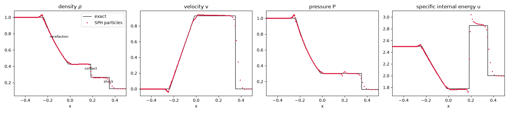
Sod’s (1978) shock tube is the standard test: gas at density and pressure \((1, 1)\) meets gas at \((0.125, 0.1)\), and the exact solution is a rarefaction, a contact discontinuity and a shock. Here 400 equal-mass particles fill the left half and 50 the right, and the SPH solution at \(t = 0.2\) is compared with the exact Riemann solution.

import matplotlib.pyplot as plt
import numpy as np

from physicskit.astro.sph import SPH1D
from physicskit.fluids.systems.compressible_flow import exact_riemann_solution

gas = SPH1D.sod_shock_tube(n_left=400)
gas.run(0.2)
x_exact = np.linspace(-0.5, 0.5, 2001)
exact = exact_riemann_solution(x_exact, 0.2)
exact_at_particles = exact_riemann_solution(gas.x, 0.2)

Density, velocity, pressure and internal energy

fig, axes = plt.subplots(1, 4, figsize=(17, 3.8))
for ax, sph_values, key, label in [
    (axes[0], gas.rho, "rho", r"density $\rho$"),
    (axes[1], gas.v, "u", "velocity v"),
    (axes[2], gas.pressure, "p", "pressure P"),
    (axes[3], gas.u, "e", "specific internal energy u"),
]:
    ax.plot(x_exact, exact[key], "k-", lw=1, label="exact")
    ax.plot(gas.x, sph_values, ".", ms=3, color="crimson", label="SPH particles")
    ax.set_xlim(-0.5, 0.5)
    ax.set_xlabel("x")
    ax.set_title(label)
axes[0].legend()
axes[0].annotate("rarefaction", (-0.18, 0.75), fontsize=8)
axes[0].annotate("contact", (0.13, 0.36), fontsize=8)
axes[0].annotate("shock", (0.3, 0.2), fontsize=8)
plt.tight_layout()
plt.show()

inner = np.abs(gas.x) < 0.45
errors = {key: np.mean(np.abs(val[inner] - exact_at_particles[key][inner])) for key, val in [("rho", gas.rho), ("p", gas.pressure)]}
plateau = (gas.x > 0.05) & (gas.x < 0.15)
print(f"mean |error|: density {errors['rho']:.4f}, pressure {errors['p']:.4f}")
print(f"post-shock velocity {gas.v[plateau].mean():.4f} (exact {float(exact['u_star']):.4f})")
print(f"energy drift {gas.energy_history[-1] / gas.energy_history[0] - 1:.2e}")

mean |error|: density 0.0068, pressure 0.0081
post-shock velocity 0.9368 (exact 0.9275)
energy drift 5.16e-04

Check

SPH follows the exact solution, apart from the smoothing of the discontinuities over a few kernel lengths and the small “wall heating” bump at the contact.

assert errors["rho"] < 0.01 and errors["p"] < 0.01
assert abs(gas.v[plateau].mean() / float(exact["u_star"]) - 1) < 0.02
assert abs(gas.energy_history[-1] / gas.energy_history[0] - 1) < 1e-3