Kepler’s laws and Newton’s inverse-square gravity

Kepler’s three empirical laws – an elliptical orbit with the Sun at one focus, equal areas swept in equal times, and \(T^2\propto a^3\) – were purely descriptive when published (1609, 1619). Newton (1687) showed they follow as mathematical consequences of a single dynamical law, the inverse-square gravitational force

\[\vec F = -\frac{G m_1 m_2}{r^2}\,\hat r,\]

with the constant of proportionality in Kepler’s third law fixed to \(\mu = GM\). This example builds one elliptical orbit with state_from_orbital_elements(), checks \(T^2\propto a^3\) numerically across several semi-major axes with orbital_period(), checks the vis-viva speed at periapsis and apoapsis against direct energy conservation, and checks Newton’s \(1/r^2\) force law directly with gravitational_acceleration().

import matplotlib.pyplot as plt
import numpy as np

from physicskit.astro.nbody import gravitational_acceleration
from physicskit.astro.orbital_mechanics import (
    orbital_period,
    state_from_orbital_elements,
    vis_viva_speed,
)

One elliptical orbit, Sun at a focus

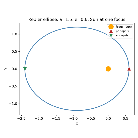
Gravitational units, \(\mu=GM=1\). An eccentricity of 0.6 makes the focus offset and the periapsis/apoapsis speed difference visually obvious.

mu = 1.0
a, e = 1.5, 0.6

nu = np.linspace(0.0, 2.0 * np.pi, 400)
r_vec = np.array([state_from_orbital_elements(a, e, 0.0, 0.0, 0.0, v, mu)[0] for v in nu])

r_peri, r_apo = a * (1.0 - e), a * (1.0 + e)

fig1, ax1 = plt.subplots(figsize=(5.5, 5.5))
ax1.plot(r_vec[:, 0], r_vec[:, 1], color="steelblue", lw=2)
ax1.plot(0, 0, "o", color="orange", ms=14, label="focus (Sun)")
ax1.plot(r_peri, 0, "^", color="firebrick", ms=9, label="periapsis")
ax1.plot(-r_apo, 0, "v", color="seagreen", ms=9, label="apoapsis")
ax1.set_xlabel("x")
ax1.set_ylabel("y")
ax1.set_title(f"Kepler ellipse, a={a}, e={e}, Sun at one focus")
ax1.set_aspect("equal")
ax1.legend(loc="upper right", fontsize=8)
fig1.tight_layout()

Kepler’s third law: \(T^2 \propto a^3\)

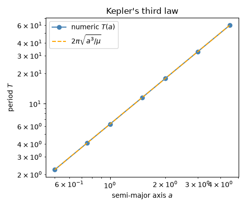
Sweep the semi-major axis over a decade and confirm orbital_period() gives exactly the \(T=2\pi\sqrt{a^3/\mu}\) scaling – \(T^2/a^3\) should be the same constant, \(4\pi^2/\mu\), at every point.

a_values = np.array([0.5, 0.75, 1.0, 1.5, 2.0, 3.0, 4.5])
T_values = np.array([orbital_period(av, mu) for av in a_values])
ratio = T_values**2 / a_values**3
expected_ratio = 4.0 * np.pi**2 / mu
print(f"T^2/a^3 for a in {a_values.tolist()}:")
print(np.round(ratio, 6))
print(f"expected 4*pi^2/mu = {expected_ratio:.6f}  (constant, as Kepler's third law demands)")

fig2, ax2 = plt.subplots(figsize=(5, 4.2))
ax2.loglog(a_values, T_values, "o-", color="steelblue", label="numeric $T(a)$")
ax2.loglog(a_values, 2 * np.pi * np.sqrt(a_values**3 / mu), "--", color="orange", label=r"$2\pi\sqrt{a^3/\mu}$")
ax2.set_xlabel("semi-major axis $a$")
ax2.set_ylabel("period $T$")
ax2.set_title("Kepler's third law")
ax2.legend()
fig2.tight_layout()

T^2/a^3 for a in [0.5, 0.75, 1.0, 1.5, 2.0, 3.0, 4.5]:
[39.478418 39.478418 39.478418 39.478418 39.478418 39.478418 39.478418]
expected 4*pi^2/mu = 39.478418  (constant, as Kepler's third law demands)

Vis-viva vs. direct energy conservation

The vis-viva equation \(v=\sqrt{\mu(2/r-1/a)}\) is itself just a restatement of energy conservation, \(v^2/2-\mu/r=-\mu/(2a)\) (the orbital binding energy per unit mass, constant around the orbit). Checking it at the two extreme points – periapsis (fastest) and apoapsis (slowest) – is the cleanest test.

v_peri = vis_viva_speed(r_peri, a, mu)
v_apo = vis_viva_speed(r_apo, a, mu)
E_peri = 0.5 * v_peri**2 - mu / r_peri
E_apo = 0.5 * v_apo**2 - mu / r_apo
E_expected = -mu / (2 * a)
print(f"\nv_periapsis = {v_peri:.6f}, v_apoapsis = {v_apo:.6f} (periapsis is faster, as area conservation requires)")
print(f"specific energy at periapsis = {E_peri:.6f}, at apoapsis = {E_apo:.6f}, expected -mu/(2a) = {E_expected:.6f}")

v_periapsis = 1.632993, v_apoapsis = 0.408248 (periapsis is faster, as area conservation requires)
specific energy at periapsis = -0.333333, at apoapsis = -0.333333, expected -mu/(2a) = -0.333333

Newton’s inverse-square law, checked directly

gravitational_acceleration() sums exactly this force pairwise; evaluated for the same Sun-planet pair at the periapsis and apoapsis distances above, the ratio of accelerations should equal \((r_{\rm apo}/r_{\rm peri})^2\).

positions_peri = np.array([[0.0, 0.0, 0.0], [r_peri, 0.0, 0.0]])
positions_apo = np.array([[0.0, 0.0, 0.0], [r_apo, 0.0, 0.0]])
masses = np.array([1.0, 1e-6])  # test-mass planet, unit-mass Sun

acc_peri = gravitational_acceleration(positions_peri, masses)[1]
acc_apo = gravitational_acceleration(positions_apo, masses)[1]
ratio_numeric = np.linalg.norm(acc_peri) / np.linalg.norm(acc_apo)
ratio_expected = (r_apo / r_peri) ** 2
print(f"\n|a(periapsis)|/|a(apoapsis)| = {ratio_numeric:.6f}, expected (r_apo/r_peri)^2 = {ratio_expected:.6f}")

plt.show()

|a(periapsis)|/|a(apoapsis)| = 16.000000, expected (r_apo/r_peri)^2 = 16.000000