Gauss’s problem: recovering orbital elements from a state vector

When Piazzi lost Ceres in the Sun’s glare after only a few weeks of observation, Gauss showed how to recover a complete set of orbital elements from as few as three observed positions and times. The modern version of the last step of that problem – given a single Cartesian state (position and velocity) at one instant, recover the six classical orbital elements \((a, e, i, \Omega, \omega, \nu)\) – is exactly what orbital_elements_from_state() does; state_from_orbital_elements() is its inverse. This example starts from a chosen (inclined, eccentric) orbit, converts to a state vector as if it were an observation, and recovers the original elements exactly – verifying the round trip in both directions, then re-derives the whole 3D orbit from the recovered elements alone.

import matplotlib.pyplot as plt
import numpy as np
from mpl_toolkits.mplot3d import Axes3D  # noqa: F401  (registers the 3D projection)

from physicskit.astro.orbital_mechanics import (
    orbital_elements_from_state,
    state_from_orbital_elements,
)

A chosen orbit, treated as ground truth

An inclined, eccentric orbit with generic (non-special) node and periapsis angles, so no accidental symmetry hides a bug in the recovery.

mu = 1.0
a_true, e_true, i_true, raan_true, argp_true, nu_true = 1.3, 0.45, 0.6, 0.9, 1.4, 2.1

r_vec, v_vec = state_from_orbital_elements(a_true, e_true, i_true, raan_true, argp_true, nu_true, mu)
print("Observed state vector (as if measured at one epoch):")
print(f"  r = {np.round(r_vec, 6)}")
print(f"  v = {np.round(v_vec, 6)}")

Observed state vector (as if measured at one epoch):
  r = [-0.476677 -1.225498 -0.26571 ]
  v = [ 0.489461 -0.504599 -0.476893]

Gauss’s inverse problem: state vector -> orbital elements

a_rec, e_rec, i_rec, raan_rec, argp_rec, nu_rec = orbital_elements_from_state(r_vec, v_vec, mu)

labels = ["a", "e", "i", "raan", "argp", "nu"]
truth = [a_true, e_true, i_true, raan_true, argp_true, nu_true]
recovered = [a_rec, e_rec, i_rec, raan_rec, argp_rec, nu_rec]
print("\nelement   true        recovered    |difference|")
for lab, t, r in zip(labels, truth, recovered):
    print(f"  {lab:5s}  {t:10.6f}  {r:10.6f}   {abs(t - r):.2e}")

element   true        recovered    |difference|
  a        1.300000    1.300000   4.44e-16
  e        0.450000    0.450000   0.00e+00
  i        0.600000    0.600000   0.00e+00
  raan     0.900000    0.900000   1.11e-16
  argp     1.400000    1.400000   4.44e-16
  nu       2.100000    2.100000   4.44e-16

Re-deriving the full orbit from the recovered elements alone

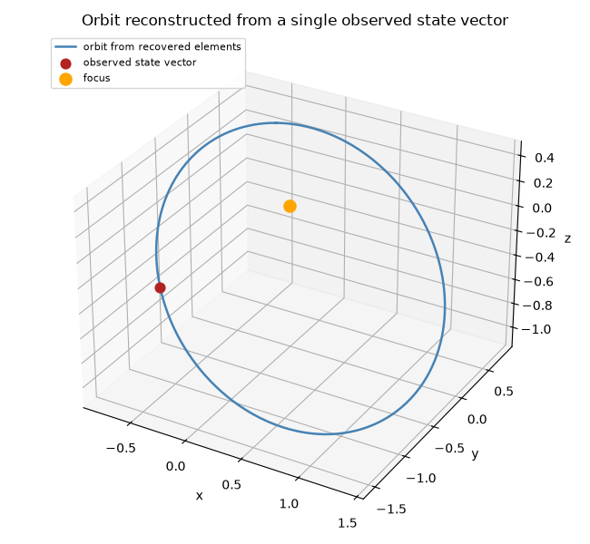
Sweep the true anomaly through a full revolution using only the recovered elements, and check that the single observed state vector lands exactly on the reconstructed orbit.

nu_sweep = np.linspace(0.0, 2.0 * np.pi, 400)
orbit_pts = np.array([state_from_orbital_elements(a_rec, e_rec, i_rec, raan_rec, argp_rec, v, mu)[0] for v in nu_sweep])

fig = plt.figure(figsize=(6.5, 6))
ax = fig.add_subplot(111, projection="3d")
ax.plot(orbit_pts[:, 0], orbit_pts[:, 1], orbit_pts[:, 2], color="steelblue", lw=1.8, label="orbit from recovered elements")
ax.scatter(*r_vec, color="firebrick", s=60, label="observed state vector")
ax.scatter(0, 0, 0, color="orange", s=90, label="focus")
ax.set_xlabel("x")
ax.set_ylabel("y")
ax.set_zlabel("z")
ax.set_title("Orbit reconstructed from a single observed state vector")
ax.legend(loc="upper left", fontsize=8)
fig.tight_layout()

plt.show()