Stellar convection and the alpha-omega magnetic dynamo

The Sun’s large-scale magnetic field is not a fossil left over from formation – it is continuously regenerated by turbulent convection acting together with differential rotation, the mechanism first proposed by Parker (1955) and still the standard textbook explanation of the 11-year solar cycle and its famous “butterfly diagram” of sunspots migrating from mid-latitudes toward the equator.

A subtlety worth being explicit about: a strictly two-dimensional, fully resolved magnetic field cannot be sustained by 2D fluid motion alone (Zeldovich’s antidynamo theorem) – real dynamo action is intrinsically three-dimensional, arising from helical turbulence that a flat, planar flow cannot produce. So this example does not attempt one self-consistent 2D “dynamo simulation” (which either wouldn’t be a real dynamo, or would silently smuggle in 3D physics). Instead, exactly as the textbook treatment splits the problem, it runs two separate, self-contained pieces:

1. A resolved 2D Boussinesq convection simulation (simulate_stellar_convection()) – turbulent convective rolls churning in a doubly periodic box, the qualitative picture of the small-scale turbulence whose unresolved 3D helical structure is, in the real Sun, the physical source of the “alpha effect” below. This piece is not itself a dynamo.

2. The linearized 1D alpha-omega mean-field dynamo equations (simulate_alpha_omega_dynamo()), in which the alpha effect and the rotational shear (the “Omega effect”) enter as prescribed coefficients rather than being derived from the convection simulation above. This piece does robustly sustain and grow a large-scale field, producing a traveling dynamo wave whose space-time diagram reproduces the solar butterfly diagram.

The two pieces are deliberately not coupled to one another.

import matplotlib.pyplot as plt
import numpy as np

from physicskit.astro.stellar_dynamo import (
    _spectral_grid_2d,  # noqa: E402  (private grid helper, for the KE diagnostic only)
    alpha_omega_growth_rate,
    alpha_omega_wave_frequency,
    dominant_mode_growth_rate,
    kinetic_energy,
    simulate_alpha_omega_dynamo,
    simulate_stellar_convection,
)
from physicskit.astro.visualizers import (
    animate_dynamo_wave,
    animate_stellar_convection,
    plot_dynamo_butterfly_diagram,
)

Part 1: 2D convective rolls

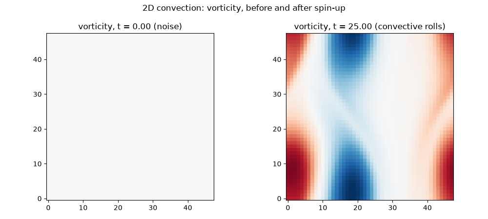
A doubly periodic Boussinesq vorticity-streamfunction-temperature system. The background stratification \(T_{eq}(y)=-\beta\cos(2\pi y/L_y)\) is unstable near its steepest gradients, and is continuously sustained against being mixed flat by the convection it drives via a Newtonian-cooling relaxation term – the standard way to force convection in a periodic box with no physical walls. Starting from tiny random noise, the flow spins up into sustained convective rolls: the kinetic energy at the end of the run is many orders of magnitude larger than at the start.

nx = ny = 48
Lx = Ly = 2 * np.pi
times_conv, omega_snaps, T_snaps = simulate_stellar_convection(nx, ny, Lx, Ly, seed=0)

_, _, KX, KY, K2 = _spectral_grid_2d(nx, ny, Lx, Ly)
KE_initial = kinetic_energy(omega_snaps[0], KX, KY, K2)
KE_final = kinetic_energy(omega_snaps[-1], KX, KY, K2)
print(f"Convective rolls: kinetic energy grew from {KE_initial:.3e} to {KE_final:.3e} (factor of {KE_final / KE_initial:.3e})")

vmax = np.abs(omega_snaps[-1]).max()
fig, axes = plt.subplots(1, 2, figsize=(10, 4.5))
axes[0].imshow(omega_snaps[0], origin="lower", cmap="RdBu_r", vmin=-vmax, vmax=vmax)
axes[0].set_title(f"vorticity, t = {times_conv[0]:.2f} (noise)")
axes[1].imshow(omega_snaps[-1], origin="lower", cmap="RdBu_r", vmin=-vmax, vmax=vmax)
axes[1].set_title(f"vorticity, t = {times_conv[-1]:.2f} (convective rolls)")
fig.suptitle("2D convection: vorticity, before and after spin-up")
fig.tight_layout()
plt.show()

Convective rolls: kinetic energy grew from 1.277e-05 to 2.061e+04 (factor of 1.613e+09)

Animating the convective rolls forming and churning.

anim_convection = animate_stellar_convection(times_conv, omega_snaps, T_snaps)
plt.show()

Part 2: the alpha-omega mean-field dynamo wave

A single Fourier mode of the linearized alpha-omega system, seeded on \(A\) alone, evolved exactly (per-Fourier-mode matrix exponential – no time-discretization error) via simulate_alpha_omega_dynamo(). Parameters are chosen so the closed-form dispersion relation \(\sigma=\sqrt{|\alpha G k|/2}-\eta k^2\) predicts robust growth.

Lx_dynamo = 2 * np.pi
nx_dynamo = 64
x = np.linspace(0, Lx_dynamo, nx_dynamo, endpoint=False)
k0 = 1.0  # m = 1 mode: k0 = 2*pi*m/Lx_dynamo
alpha, shear, eta = 1.0, 5.0, 0.05

A0 = 1e-3 * np.cos(k0 * x)
B0 = np.zeros_like(A0)

dt = 0.01
n_steps = 600
save_every = 5
times_dynamo, A_snaps, B_snaps = simulate_alpha_omega_dynamo(A0, B0, alpha, shear, eta, Lx_dynamo, dt, n_steps, save_every)

sigma_predicted = alpha_omega_growth_rate(alpha, shear, k0, eta)
sigma_observed = dominant_mode_growth_rate(B_snaps, dt_save=dt * save_every)
print(
    f"Alpha-omega dynamo growth rate: analytic sigma = {sigma_predicted:.6f}, "
    f"numerically-fit sigma = {sigma_observed:.6f} "
    f"(relative difference {abs(sigma_observed - sigma_predicted) / sigma_predicted:.2%})"
)

Alpha-omega dynamo growth rate: analytic sigma = 1.531139, numerically-fit sigma = 1.531130 (relative difference 0.00%)

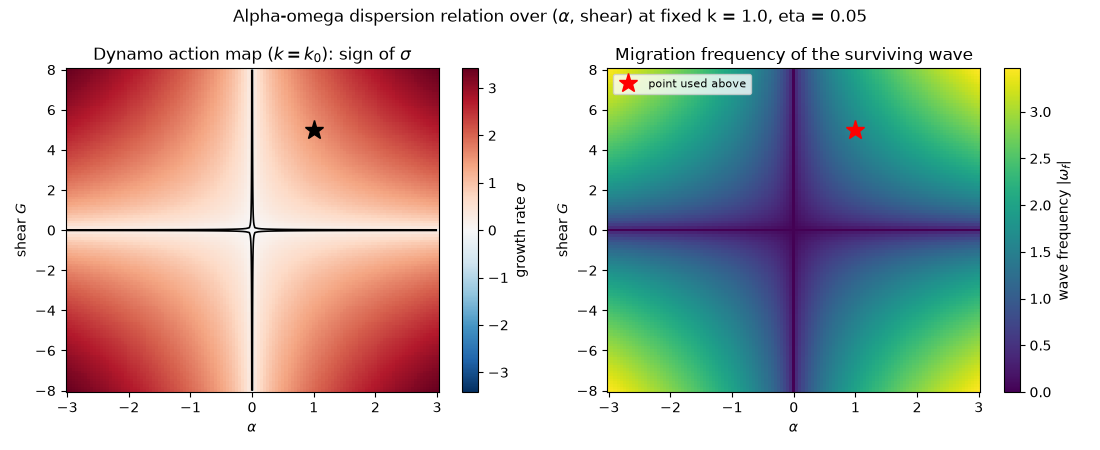
The dynamo action map: growth rate and wave frequency over (alpha, shear)

The single (alpha, shear, k0) point checked above sits somewhere in a much larger two-parameter landscape. The closed-form dispersion relation is cheap to evaluate everywhere, so scan it over a grid of alpha-effect strength and rotational shear (at the fixed k0 and eta used in the simulation) to map out where the alpha-omega mechanism actually sustains a growing wave (\(\sigma>0\), alpha_omega_growth_rate()) versus where Ohmic diffusion wins and the mode simply decays, and how fast the surviving wave migrates (alpha_omega_wave_frequency()). With the small diffusivity used here, the decay region (pale/blue, bounded by the black \(\sigma=0\) contour) is squeezed into a thin sliver hugging the two axes: growth needs both a nonzero alpha effect and nonzero shear (neither ingredient alone can sustain a dynamo – consistent with the antidynamo reasoning in this example’s module docstring), but once both are present at all, growth follows almost everywhere.

alpha_range = np.linspace(-3.0, 3.0, 121)
shear_range = np.linspace(-8.0, 8.0, 121)
Alpha, Shear = np.meshgrid(alpha_range, shear_range)

sigma_map = alpha_omega_growth_rate(Alpha, Shear, k0, eta)
omega_map = alpha_omega_wave_frequency(Alpha, Shear, k0)

fig_map, (ax_sigma, ax_omega) = plt.subplots(1, 2, figsize=(11, 4.5))

sigma_lim = np.abs(sigma_map).max()
im_sigma = ax_sigma.pcolormesh(Alpha, Shear, sigma_map, cmap="RdBu_r", vmin=-sigma_lim, vmax=sigma_lim, shading="auto")
ax_sigma.contour(Alpha, Shear, sigma_map, levels=[0.0], colors="k", linewidths=1.2)
fig_map.colorbar(im_sigma, ax=ax_sigma, label=r"growth rate $\sigma$")
ax_sigma.plot(alpha, shear, "k*", ms=14)
ax_sigma.set_xlabel(r"$\alpha$")
ax_sigma.set_ylabel("shear $G$")
ax_sigma.set_title(r"Dynamo action map ($k=k_0$): sign of $\sigma$")

im_omega = ax_omega.pcolormesh(Alpha, Shear, omega_map, cmap="viridis", shading="auto")
fig_map.colorbar(im_omega, ax=ax_omega, label=r"wave frequency $|\omega_f|$")
ax_omega.plot(alpha, shear, "r*", ms=14, label="point used above")
ax_omega.set_xlabel(r"$\alpha$")
ax_omega.set_ylabel("shear $G$")
ax_omega.set_title("Migration frequency of the surviving wave")
ax_omega.legend(loc="upper left", fontsize=8)
fig_map.suptitle(f"Alpha-omega dispersion relation over ($\\alpha$, shear) at fixed k = {k0}, eta = {eta}")
fig_map.tight_layout()

Animating the migrating, growing dynamo wave.

anim_dynamo = animate_dynamo_wave(times_dynamo, A_snaps, B_snaps, x)
plt.show()

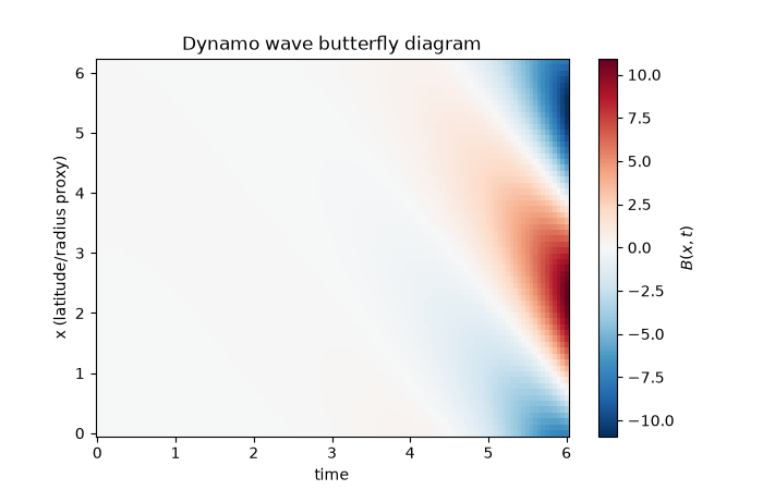
The butterfly diagram: a static space-time summary of the same wave, showing the diagonal migrating stripes that are the whole point of the alpha-omega mechanism – the same phenomenology behind the real Sun’s sunspot-latitude butterfly diagram.

fig_bf, ax_bf = plot_dynamo_butterfly_diagram(times_dynamo, B_snaps, x)
plt.show()