Building a Custom System with the Low-Level Integrators

Every built-in continuous system in physicskit.chaos.systems.continuous follows the same recipe: a module-level Numba @njit right-hand-side function with signature rhs(state, t, params) -> ndarray, wrapped by a physicskit.chaos.core.base_system.DynamicalSystem subclass whose trajectory() method calls physicskit.chaos.core.integrators.rk4_integrate(). This example follows that same recipe to add a new system – the Van der Pol oscillator – that is not one of the built-ins, and then shows the even more low-level path of calling an integrator directly on a bare right-hand-side function with no wrapper class at all.

from __future__ import annotations

import matplotlib.pyplot as plt
import numpy as np
from numba import njit
from numpy.typing import NDArray

from physicskit.chaos.core.base_system import DynamicalSystem
from physicskit.chaos.core.integrators import leapfrog_integrate, rk4_integrate

Recipe 1: a full DynamicalSystem subclass

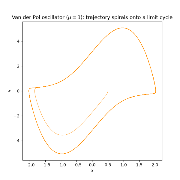
This is the same pattern used by physicskit.chaos.systems.continuous.Lorenz and friends – it plugs into every other physicskit.chaos tool (the Lyapunov metrics, the divergence visualizer, etc.) that expects a DynamicalSystem. The system built here, the Van der Pol oscillator, is the classic model of a relaxation oscillator – a self-sustaining electrical circuit oscillation (originally a vacuum-tube circuit) with amplitude-dependent damping:

\[\ddot{x} - \mu (1 - x^2) \dot{x} + x = 0,\]

or, as the first-order system in \((x, v)\) actually integrated, \(\dot{x} = v\), \(\dot{v} = \mu(1-x^2)v - x\). The nonlinear damping term pumps energy in when \(|x| < 1\) (negative damping) and removes it when \(|x| > 1\) (positive damping), so trajectories from any nonzero initial condition spiral onto the same stable limit cycle regardless of amplitude.

@njit(cache=True)
def _van_der_pol_rhs(state: NDArray[np.float64], t: float, params: NDArray[np.float64]) -> NDArray[np.float64]:
    r"""Van der Pol vector field ``dx/dt = f(x, t; mu)``."""
    mu = params[0]
    x, v = state[0], state[1]
    out = np.empty(2)
    out[0] = v
    out[1] = mu * (1.0 - x * x) * v - x
    return out


class VanDerPol(DynamicalSystem):
    r"""The Van der Pol oscillator: a relaxation oscillator with a stable limit cycle."""

    dim = 2

    def __init__(self, mu: float = 3.0):
        self.mu = float(mu)

    @property
    def params(self) -> NDArray[np.float64]:
        return np.array([self.mu])

    def rhs(self, state: NDArray[np.float64], t: float) -> NDArray[np.float64]:
        return np.asarray(_van_der_pol_rhs(np.asarray(state, dtype=np.float64), t, self.params))

    def initial_state(self) -> NDArray[np.float64]:
        return np.array([0.5, 0.0])

    def trajectory(self, state0=None, t0: float = 0.0, dt: float = 0.01, n_steps: int = 5000):
        state0 = self.initial_state() if state0 is None else np.asarray(state0, dtype=np.float64)
        return rk4_integrate(_van_der_pol_rhs, state0, t0, dt, n_steps, self.params)


system = VanDerPol(mu=3.0)
t, states = system.trajectory(n_steps=5000, dt=0.01)

fig, ax = plt.subplots(figsize=(6, 6))
ax.plot(states[:, 0], states[:, 1], lw=0.6, color="darkorange")
ax.set_xlabel("x")
ax.set_ylabel("v")
ax.set_title(r"Van der Pol oscillator ($\mu=3$): trajectory spirals onto a limit cycle")

Text(0.5, 1.0, 'Van der Pol oscillator ($\\mu=3$): trajectory spirals onto a limit cycle')

Recipe 2: calling an integrator directly, with no wrapper class

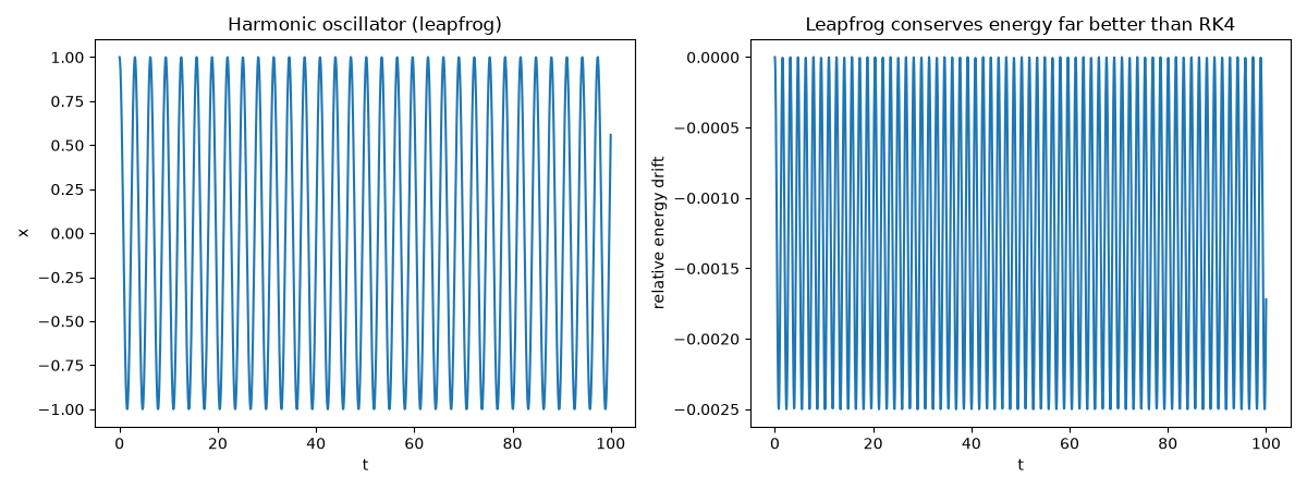
For quick experiments you don’t need a full class at all: any Numba @njit function with signature f(state, t, params) -> ndarray can be handed straight to rk4_integrate(). Here we integrate a plain (undamped, undriven) simple harmonic oscillator,

\[\ddot{x} = -\omega^2 x,\]

with the symplectic leapfrog integrator instead, which conserves the conserved energy \(E = \tfrac{1}{2}v^2 + \tfrac{1}{2}\omega^2 x^2\) far better than RK4 over long integrations because it exactly preserves phase-space volume.

@njit(cache=True)
def _harmonic_force(pos: NDArray[np.float64], t: float, params: NDArray[np.float64]) -> NDArray[np.float64]:
    """Restoring force ``-omega^2 * x`` for a simple harmonic oscillator."""
    omega = params[0]
    return -(omega**2) * pos


omega = 2.0
pos0 = np.array([1.0])
vel0 = np.array([0.0])
t2, positions, velocities = leapfrog_integrate(_harmonic_force, pos0, vel0, 0.0, 0.05, 2000, np.array([omega]))

energy = 0.5 * velocities[:, 0] ** 2 + 0.5 * omega**2 * positions[:, 0] ** 2

fig2, (ax1, ax2) = plt.subplots(1, 2, figsize=(12, 4.5))
ax1.plot(t2, positions[:, 0])
ax1.set_xlabel("t")
ax1.set_ylabel("x")
ax1.set_title("Harmonic oscillator (leapfrog)")
ax2.plot(t2, (energy - energy[0]) / energy[0])
ax2.set_xlabel("t")
ax2.set_ylabel("relative energy drift")
ax2.set_title("Leapfrog conserves energy far better than RK4")
fig2.tight_layout()

plt.show()