Truncated Circle Billiard (Mixed Phase Space)

A billiard particle moves in a straight line at constant speed inside a closed boundary and undergoes specular reflection, \(\mathbf{v}' = \mathbf{v} - 2(\mathbf{v}\cdot\mathbf{n})\,\mathbf{n}\), whenever it strikes the boundary. This billiard’s boundary keeps the major arc of a circle of radius \(r\), \(x^2+y^2=r^2\), and closes it off with a straight chord at \(x = r - c\), where \(c\) (cut) is how far the chord is cut in from the circle’s edge. Slicing this flat chord off a circular billiard breaks integrability without making the system fully chaotic: depending on how large \(c\) is, the Poincare section shows a mix of regular invariant curves (surviving islands near the untouched part of the circle) and a chaotic sea near the chord. This “mixed” behavior sits between the fully integrable Circle/Rectangle billiards and the fully chaotic Sinai/Stadium billiards.

import matplotlib.pyplot as plt
import numpy as np

from physicskit.chaos.systems.billiards import TruncatedCircleBilliard
from physicskit.chaos.visualizers.dynamic_plots import animate_billiard_trajectory
from physicskit.chaos.visualizers.phase_space import plot_billiard_trajectory, plot_poincare_section

billiard = TruncatedCircleBilliard(radius=1.0, cut=0.3)

Animation

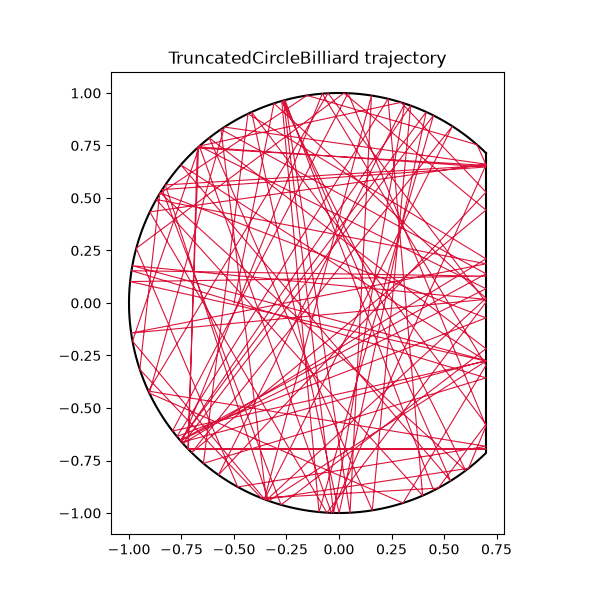
Watch for the ray alternating between long, regular runs around the untouched circular arc and short, erratic bounces near the flat chord.

anim = animate_billiard_trajectory(billiard, pos=billiard.sample_interior_point(), vel=(0.2, 1.0), n_bounces=100, interval=50)

plt.show()

To save the animation to a file instead of (or in addition to) displaying it interactively, use e.g.:

anim.save("truncated_circle_billiard_animation.gif", writer="pillow", fps=25)

Trajectory

fig, ax = plot_billiard_trajectory(billiard, pos=billiard.sample_interior_point(), vel=np.array([0.2, 1.0]), n_bounces=100)

Poincare section

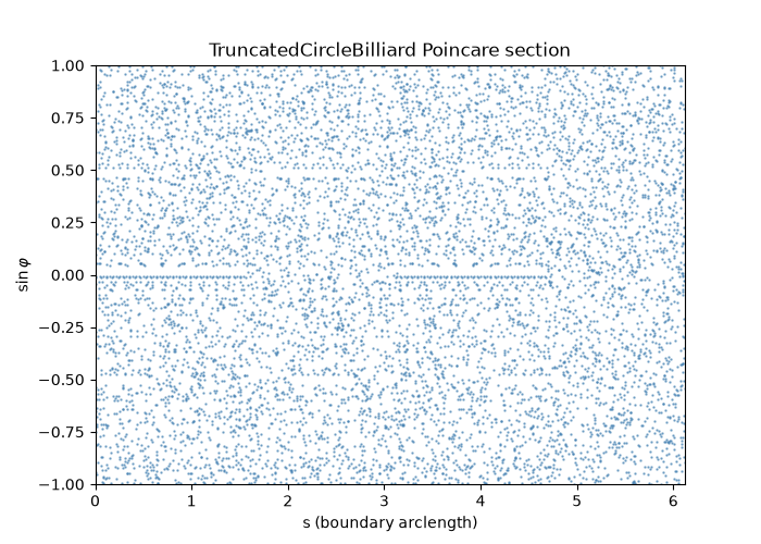
Look for a mix of smooth horizontal-ish bands (regular islands, inherited from the untouched circular arc) alongside a scattered chaotic sea (from rays that repeatedly strike near the flat chord).

fig, ax = plot_poincare_section(billiard, n_rays=40, n_bounces=200)

plt.show()

Watching the mix change: a sweep over the cut depth

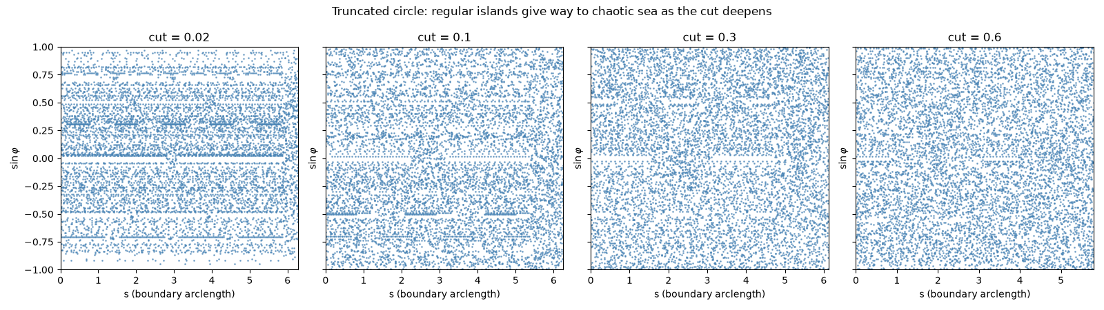
cut = 0.3 above is just one point along a continuum from “barely truncated” to “truncated almost in half”. Building a fresh TruncatedCircleBilliard at each of several cut values and plotting each one’s Poincare section side by side (the same plot_poincare_section() used above, just swept) shows the regular-to-chaotic transition directly: a razor-thin chord leaves the section almost entirely covered by the circle’s smooth invariant curves, with only a sliver of chaotic sea near sin(phi) = 0; as the cut deepens, that chaotic sliver eats into more and more of the section, squeezing the surviving regular islands into thinner bands near the top and bottom.

cut_values = [0.02, 0.1, 0.3, 0.6]
fig2, axes2 = plt.subplots(1, len(cut_values), figsize=(16, 4.5), sharey=True)
for ax_i, cut in zip(axes2, cut_values):
    plot_poincare_section(TruncatedCircleBilliard(radius=1.0, cut=cut), n_rays=40, n_bounces=200, ax=ax_i, s=1.0, seed=0)
    ax_i.set_title(f"cut = {cut}")
fig2.suptitle("Truncated circle: regular islands give way to chaotic sea as the cut deepens")
fig2.tight_layout()

plt.show()