Kuramoto synchronization: the onset at a critical coupling

Kuramoto’s model couples \(N\) phase oscillators with natural frequencies \(\omega_i\) drawn from \(g(\omega)\), every one to every other,

\[\dot\theta_i = \omega_i + \frac{K}{N}\sum_j \sin(\theta_j - \theta_i), \qquad r e^{i\psi} = \frac1N \sum_j e^{i\theta_j}.\]

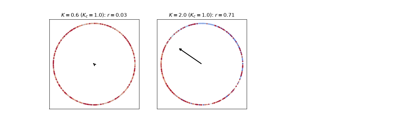
Below a critical coupling \(K_c = 2/(\pi g(0))\) the phases stay incoherent and \(r \approx 0\). Above it a synchronized cluster forms spontaneously, and for a Lorentzian \(g\) of half-width \(\gamma\) the order parameter is exactly

\[r = \sqrt{1 - K_c/K}, \qquad K_c = 2\gamma.\]

This example integrates \(N = 2000\) oscillators, shows the phases locking on the unit circle, and measures \(r(K)\) across the onset.

import matplotlib.pyplot as plt
import numpy as np

from physicskit.chaos.systems.synchronization import Kuramoto, kuramoto_order_parameter_lorentzian

gamma = 0.5
N = 2000

Phases on the unit circle, below and above onset

fig = plt.figure(figsize=(13, 4.2))
for panel, K in enumerate([0.6, 2.0]):
    model = Kuramoto(N, K=K, gamma=gamma)
    _, states = model.trajectory(dt=0.05, n_steps=2000)
    theta = states[-1]
    r = model.order_parameter(theta)
    ax = fig.add_subplot(1, 3, panel + 1)
    ax.plot(np.cos(np.linspace(0, 2 * np.pi, 200)), np.sin(np.linspace(0, 2 * np.pi, 200)), color="gray", lw=0.5)
    ax.scatter(np.cos(theta), np.sin(theta), c=np.clip(model.omega, -3, 3), cmap="coolwarm", s=4)
    z = np.mean(np.exp(1j * theta))
    ax.annotate("", xy=(z.real, z.imag), xytext=(0, 0), arrowprops={"arrowstyle": "->", "lw": 2})
    ax.set_title(rf"$K = {K}$ ($K_c = {model.critical_coupling}$): $r = {r:.2f}$")
    ax.set_aspect("equal")
    ax.set_xticks([])
    ax.set_yticks([])

The order parameter across the transition

Each point is the time average of \(r(t)\) after the transient, from incoherent initial phases.

K_values = np.linspace(0.2, 4.0, 20)
r_measured = np.array([Kuramoto(N, K=K, gamma=gamma).order_parameter_series(t_max=200.0, seed=1)[-1000:].mean() for K in K_values])
K_fine = np.linspace(0.0, 4.0, 400)
ax = fig.add_subplot(1, 3, 3)
ax.plot(K_fine, kuramoto_order_parameter_lorentzian(K_fine, gamma), "k-", label=r"$\sqrt{1 - 2\gamma/K}$")
ax.plot(K_values, r_measured, "o", color="crimson", label=f"N = {N}")
ax.axvline(2 * gamma, color="gray", ls="--", lw=0.8)
ax.set_xlabel("coupling K")
ax.set_ylabel("order parameter r")
ax.set_title(rf"Lorentzian $g(\omega)$, $\gamma = {gamma}$")
ax.legend()
plt.tight_layout()
plt.show()

above = K_values > 1.3 * 2 * gamma
err = np.max(np.abs(r_measured[above] - kuramoto_order_parameter_lorentzian(K_values[above], gamma)))
print(f"max |r - sqrt(1 - Kc/K)| above onset: {err:.3f}")

max |r - sqrt(1 - Kc/K)| above onset: 0.001

Check

Above onset the measured order parameter follows Kuramoto’s closed form; well below it, only the \(O(N^{-1/2})\) finite-size remnant is left.

assert err < 0.02
assert np.all(r_measured[K_values < 0.7 * 2 * gamma] < 0.1)