Euler’s Disk: a finite-time singularity on a tabletop

Spin a disk and set it rolling flat on a table and it settles into a shuddering near-steady state described, at each instant, by just its inclination angle \(\theta\) (between the disk plane and the table) and precession angle \(\phi\) (the azimuthal angle of the rolling contact point). Its contact point precesses faster and faster – the characteristic rattle rising in pitch – right up until the disk suddenly stops: a finite-time singularity. Rather than committing to one first-principles dissipation mechanism (viscous air drag vs. rolling friction are both argued for in the literature; see the history page), EulersDisk uses a reduced phenomenological pair of ODEs,

\[\dot\theta = -\frac{\text{decay\_rate}}{\theta}, \qquad \dot\phi = \frac{\text{precession\_const}}{\theta} ,\]

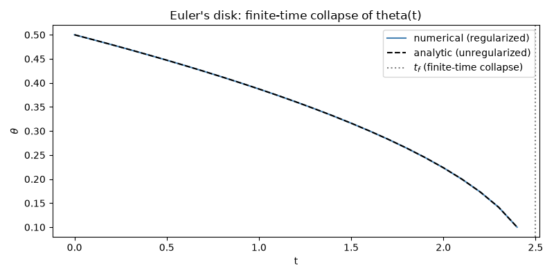
in which both the precession rate and the (implied) dissipation rate diverge as \(\theta \to 0\), reproducing the same qualitative finite-time collapse. Ignoring the regularizing floor near \(\theta = 0\), the first equation integrates in closed form to \(\theta(t) = \sqrt{\theta_0^2 - 2\,\text{decay\_rate}\cdot t}\), vanishing at the finite collapse time \(t_f = \theta_0^2 / (2\,\text{decay\_rate})\).

import matplotlib.pyplot as plt

from physicskit.classical.systems.rotations import EulersDisk, eulers_disk_theta_analytic
from physicskit.classical.visualizers.animations import animate_eulers_disk

theta0, decay_rate = 0.5, 0.05
t_f = theta0**2 / (2.0 * decay_rate)
system = EulersDisk(theta0=theta0, decay_rate=decay_rate, precession_const=1.5)

# Stop just short of the (regularized) collapse time -- theta keeps
# decreasing past zero once floored, which is no longer physically
# meaningful.
result = system.integrate((0.0, 0.98 * t_f), dt=1e-1, method="implicit_midpoint")

Animation: the contact point spiraling inward

Watch the contact point spiral toward the center and precess faster and faster as theta collapses toward zero.

anim = animate_eulers_disk(system, result, interval=30, trail=600)

plt.show()

To save the animation to a file instead of (or in addition to) displaying it interactively, use e.g.:

anim.save("eulers_disk_animation.gif", writer="pillow", fps=30)

Numerical vs. analytic collapse

The regularized numerical theta(t) tracks the exact, unregularized closed-form solution theta(t) = sqrt(theta0^2 - 2*decay_rate*t) almost all the way to the finite collapse time t_f.

theta_exact = eulers_disk_theta_analytic(result.t, theta0, decay_rate)

fig, ax = plt.subplots(figsize=(8, 4))
ax.plot(result.t, result.y[:, 0], label="numerical (regularized)", color="steelblue")
ax.plot(result.t, theta_exact, "k--", label="analytic (unregularized)")
ax.axvline(t_f, color="gray", ls=":", label=r"$t_f$ (finite-time collapse)")
ax.set_xlabel("t")
ax.set_ylabel(r"$\theta$")
ax.set_title("Euler's disk: finite-time collapse of theta(t)")
ax.legend()
fig.tight_layout()

plt.show()