Anderson Localization: Disorder Halts Diffusion

Philip Anderson showed that random onsite disorder, at any nonzero strength, exponentially localizes every eigenstate of a 1D tight-binding chain (anderson_chain_hamiltonian()). The inverse participation ratio (inverse_participation_ratio()) distinguishes extended states (\(\text{IPR}\sim 1/N\)) from localized ones (\(\text{IPR}=O(1)\)), and localization_length() extracts the decay length \(\xi\) directly from an eigenstate’s envelope.

import matplotlib.pyplot as plt
import numpy as np

from physicskit.condensed.anderson_localization import (
    anderson_chain_hamiltonian,
    inverse_participation_ratio,
    localization_length,
)

A mid-spectrum eigenstate: extended (clean) vs localized (disordered)

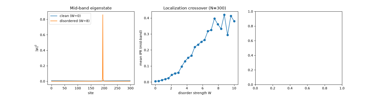
In a clean chain the mid-band eigenstate spreads over the entire system. Turning on strong disorder collapses it onto a handful of sites.

n_sites = 300
H_clean = anderson_chain_hamiltonian(n_sites=n_sites, disorder_strength=0.0)
H_disordered = anderson_chain_hamiltonian(n_sites=n_sites, disorder_strength=8.0, seed=0)

_, vecs_clean = np.linalg.eigh(H_clean)
eigs_dis, vecs_disordered = np.linalg.eigh(H_disordered)

psi_clean = vecs_clean[:, n_sites // 2]
psi_disordered = vecs_disordered[:, n_sites // 2]

ipr_clean = inverse_participation_ratio(psi_clean)
ipr_disordered = inverse_participation_ratio(psi_disordered)
xi = localization_length(psi_disordered)
print(f"clean chain:      IPR = {ipr_clean:.5f}  (~1/N = {1 / n_sites:.5f})")
print(f"disordered chain: IPR = {ipr_disordered:.5f}, localization length xi = {xi:.2f}")

clean chain:      IPR = 0.00498  (~1/N = 0.00333)
disordered chain: IPR = 0.74410, localization length xi = 1.70

IPR vs disorder strength: the localization crossover

Averaged over disorder realizations, the mid-band IPR rises steeply from its clean, near-zero value as disorder turns on – in 1D, arbitrarily weak disorder eventually localizes every state as the chain grows, but a finite chain shows a smooth crossover.

disorder_values = np.linspace(0.0, 10.0, 25)
n_realizations = 10
mean_ipr = []
for W in disorder_values:
    iprs = []
    for seed in range(n_realizations):
        H = anderson_chain_hamiltonian(n_sites=n_sites, disorder_strength=W, seed=seed)
        _, vecs = np.linalg.eigh(H)
        iprs.append(inverse_participation_ratio(vecs[:, n_sites // 2]))
    mean_ipr.append(np.mean(iprs))

fig, axes = plt.subplots(1, 3, figsize=(16, 4))

axes[0].plot(np.abs(psi_clean) ** 2, label="clean (W=0)", lw=1.5)
axes[0].plot(np.abs(psi_disordered) ** 2, label="disordered (W=8)", lw=1.5)
axes[0].set_xlabel("site")
axes[0].set_ylabel(r"$|\psi_i|^2$")
axes[0].set_title("Mid-band eigenstate")
axes[0].legend()

axes[1].plot(disorder_values, mean_ipr, "o-")
axes[1].set_xlabel("disorder strength W")
axes[1].set_ylabel("mean IPR (mid-band)")
axes[1].set_title(f"Localization crossover (N={n_sites})")

Text(0.5, 1.0, 'Localization crossover (N=300)')

Every eigenstate localizes somewhere different

The single mid-band state above is one row of a much larger picture: at strong disorder, every eigenstate of the same disordered chain is independently localized, each to its own handful of sites. Stacking \(|\psi_n(x)|^2\) for every eigenstate n (sorted by energy) into one image makes that collective structure visible at a glance – a scatter of bright, narrow spots rather than the smooth bands a clean chain’s extended eigenstates would produce.

density_all = np.abs(vecs_disordered) ** 2  # shape (site, eigenstate index)

# A linear color scale only shows each state's single brightest pixel --
# every eigenstate is normalized to 1, so nearly all of that weight sits
# on one or two sites and the exponentially decaying tails (the actual
# signature of the localization length xi) are far too faint to see next
# to that peak. A log scale, floored well above floating-point noise,
# recovers those tails as visible halos around each bright core.
im = axes[2].imshow(
    density_all.T,
    aspect="auto",
    origin="lower",
    cmap="inferno",
    norm=plt.matplotlib.colors.LogNorm(vmin=1e-3, vmax=density_all.max(), clip=True),
    extent=[0, n_sites, eigs_dis[0], eigs_dis[-1]],
)
axes[2].set_xlabel("site")
axes[2].set_ylabel("energy (eigenstate sorted by E)")
axes[2].set_title(f"Every eigenstate, W={8.0:.0f}: all independently localized")
fig.colorbar(im, ax=axes[2], label=r"$|\psi_n(x)|^2$ (log scale)", shrink=0.85)

fig.tight_layout()