Ginzburg-Landau Theory: Healing Length and Type I vs Type II

Ginzburg and Landau described superconductivity with a free-energy functional of a complex order parameter alone, no microscopic pairing mechanism required. Minimizing it gives an equilibrium condensate density \(|\psi_0|^2=-a/b\) (gl_equilibrium_order_parameter()) below the transition, and two length scales – the coherence length \(\xi\) (gl_coherence_length()) and the penetration depth \(\lambda\) (gl_penetration_depth()) – whose ratio, the Ginzburg-Landau parameter \(\kappa\) (ginzburg_landau_parameter()), alone decides Type I vs Type II behavior.

import matplotlib.pyplot as plt
import numpy as np

from physicskit.condensed.ginzburg_landau import (
    ginzburg_landau_parameter,
    gl_coherence_length,
    gl_equilibrium_order_parameter,
    gl_free_energy_density,
    gl_order_parameter_profile,
    gl_penetration_depth,
)

The free energy’s double-well shape below the transition

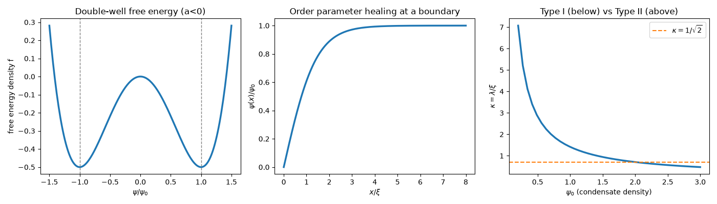
For a < 0, f(psi) has degenerate minima at psi = +-psi0 rather than the single minimum psi=0 of the normal state (a > 0).

a, b = -1.0, 1.0
psi0 = gl_equilibrium_order_parameter(a, b)
psi_range = np.linspace(-1.5 * psi0, 1.5 * psi0, 200)
free_energy = [gl_free_energy_density(psi, a, b) for psi in psi_range]
print(f"equilibrium order parameter psi0 = {psi0:.4f}")

equilibrium order parameter psi0 = 1.0000

The order parameter heals from a boundary over the coherence length

Pinned to zero at a boundary (e.g. a normal-superconducting interface), the order parameter recovers its bulk value over a few coherence lengths – the exact analytic solution gl_order_parameter_profile().

xi = gl_coherence_length(a=a)
x = np.linspace(0, 8 * xi, 300)
profile = gl_order_parameter_profile(x, xi)

Type I vs Type II: the Ginzburg-Landau parameter kappa

A denser condensate screens magnetic fields over a shorter penetration depth. Sweeping psi0 sweeps kappa=lambda/xi across the 1/sqrt(2) Type I / Type II boundary.

psi0_values = np.linspace(0.2, 3.0, 40)
kappas = [ginzburg_landau_parameter(xi, gl_penetration_depth(psi0=p)) for p in psi0_values]
kappa_c = 1.0 / np.sqrt(2)

fig, axes = plt.subplots(1, 3, figsize=(14, 4))

axes[0].plot(psi_range / psi0, free_energy, lw=2.5)
axes[0].axvline(1.0, color="gray", ls="--", lw=1)
axes[0].axvline(-1.0, color="gray", ls="--", lw=1)
axes[0].set_xlabel(r"$\psi/\psi_0$")
axes[0].set_ylabel("free energy density f")
axes[0].set_title("Double-well free energy (a<0)")

axes[1].plot(x / xi, profile, lw=2.5)
axes[1].set_xlabel(r"$x/\xi$")
axes[1].set_ylabel(r"$\psi(x)/\psi_0$")
axes[1].set_title("Order parameter healing at a boundary")

axes[2].plot(psi0_values, kappas, lw=2.5)
axes[2].axhline(kappa_c, color="C1", ls="--", label=r"$\kappa=1/\sqrt{2}$")
axes[2].set_xlabel(r"$\psi_0$ (condensate density)")
axes[2].set_ylabel(r"$\kappa=\lambda/\xi$")
axes[2].set_title("Type I (below) vs Type II (above)")
axes[2].legend()

fig.tight_layout()