Landau’s 1930 Solution: Discrete Levels from a Continuous Field

Lev Landau solved the quantum mechanics of a charged particle in a uniform magnetic field \(B\) directly, with no lattice involved: the classically continuous cyclotron motion collapses into equally spaced, macroscopically degenerate levels \(E_n = \hbar\omega_c(n+1/2)\), landau_level_energies(). Each level holds \(n_B\) states per unit area, landau_degeneracy(), growing linearly with \(B\) – the origin of Landau diamagnetism, and the reason a 2D electron gas’s Landau-level filling factor \(\nu=n_e/n_B\) (filling_factor()) is the natural variable of the quantum Hall effect.

import matplotlib.pyplot as plt
import numpy as np

from physicskit.condensed.landau_levels import (
    filling_factor,
    landau_degeneracy,
    landau_density_of_states,
    landau_level_energies,
)

Equally spaced levels, exactly the harmonic oscillator spectrum

With \(\hbar=m=e=1\), a field \(B=1\) gives cyclotron frequency \(\omega_c=1\) and levels at half-integers – identical to a harmonic oscillator, with the field itself playing the role of the spring constant.

B = 1.0
n_max = 6
energies = landau_level_energies(n_max=n_max, B=B)
print(f"Landau levels at B={B}: {np.round(energies, 3)}")
print(f"level spacing (should be constant, = hbar*omega_c=1): {np.round(np.diff(energies), 6)}")

Landau levels at B=1.0: [0.5 1.5 2.5 3.5 4.5 5.5 6.5]
level spacing (should be constant, = hbar*omega_c=1): [1. 1. 1. 1. 1. 1.]

Degeneracy per unit area grows linearly with the field

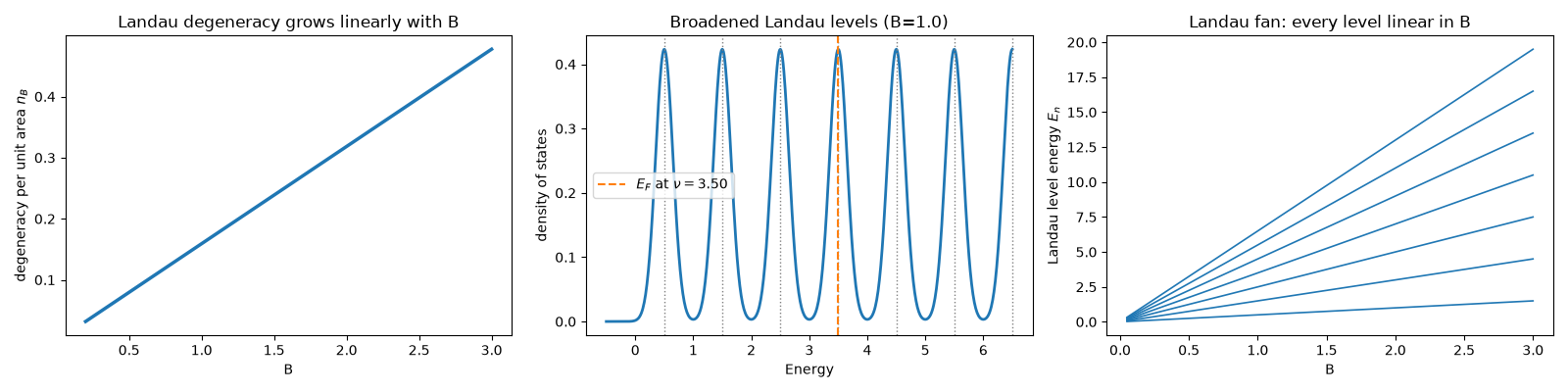
Doubling B packs twice as many states into each level – the microscopic reason a stronger field makes the quantum Hall plateaus (fixed integer filling factor) occur at lower electron density.

B_values = np.linspace(0.2, 3.0, 30)
degeneracies = [landau_degeneracy(area=1.0, B=B) for B in B_values]

Disorder-broadened density of states and the filling factor

A real 2D electron gas’s Landau levels are broadened by disorder into Gaussian peaks (landau_density_of_states()). For a fixed electron density, the filling factor marks how many levels are (on average) filled.

B_fixed = 1.0
density = 3.5 / (2 * np.pi)  # chosen to land nu midway through the third level
nu = filling_factor(density=density, B=B_fixed)
print(f"electron density={density}, B={B_fixed} -> filling factor nu={nu:.3f}")

E_grid = np.linspace(-0.5, 6.5, 600)
dos = landau_density_of_states(E_grid, B=B_fixed, n_max=6, broadening=0.15)

electron density=0.5570423008216338, B=1.0 -> filling factor nu=3.500

The Landau fan: level energies rising linearly with the field

Each level’s energy \(E_n(B) = (n+1/2)\hbar\omega_c(B)\) is exactly linear in \(B\) (with \(m=e=\hbar=1\)), so sweeping the field and stacking every landau_level_energies() call into one image traces out a fan of straight lines radiating from the origin – the standard experimental “Landau fan diagram” used to read the cyclotron mass directly off the fan’s slope.

B_fan = np.linspace(0.05, 3.0, 200)
fan_energies = np.array([landau_level_energies(n_max=6, B=B) for B in B_fan])

fig, axes = plt.subplots(1, 3, figsize=(16, 4))

ax = axes[0]
ax.plot(B_values, degeneracies, lw=2.5)
ax.set_xlabel("B")
ax.set_ylabel(r"degeneracy per unit area $n_B$")
ax.set_title("Landau degeneracy grows linearly with B")

ax = axes[1]
ax.plot(E_grid, dos, lw=2)
for n in range(7):
    ax.axvline(n + 0.5, color="gray", ls=":", lw=1)
ax.axvline(nu * 1.0, color="C1", ls="--", label=rf"$E_F$ at $\nu={nu:.2f}$")
ax.set_xlabel("Energy")
ax.set_ylabel("density of states")
ax.set_title(f"Broadened Landau levels (B={B_fixed})")
ax.legend()

ax = axes[2]
ax.plot(B_fan, fan_energies, color="C0", lw=1.2)
ax.set_xlabel("B")
ax.set_ylabel("Landau level energy $E_n$")
ax.set_title("Landau fan: every level linear in B")

fig.tight_layout()