The Fractional Quantum Hall Effect: Laughlin’s Correlation Hole

Tsui, Stormer, and Gossard’s 1982 discovery of a Hall plateau at filling \(\nu=1/3\) – a fraction the single-particle Landau-level picture behind the integer effect cannot explain, since a partially filled Landau level is gapless without interactions – was explained the following year by Laughlin’s many-body trial wavefunction,

\[\Psi_m(z_1,\dots,z_N) = \prod_{i<j}(z_i-z_j)^m\, e^{-\sum_i|z_i|^2/4\ell_B^2}, \qquad m=3 \text{ for } \nu=1/3.\]

\(|\Psi_m|^2\) doubles as the Boltzmann weight of a classical 2D plasma (Laughlin’s “plasma analogy”), letting laughlin_metropolis_sweep() sample it directly with ordinary Metropolis Monte Carlo – no diagonalization of any kind. The resulting pair correlation function (laughlin_pair_correlation()) shows the wavefunction’s defining feature: particles actively avoid each other far more strongly than Pauli exclusion alone requires, a “correlation hole” that vanishes at zero separation and whose quasihole excitations carry the fractional charge \(e/m\).

import matplotlib.pyplot as plt
import numpy as np

from physicskit.condensed.laughlin import laughlin_metropolis_sweep, laughlin_pair_correlation, laughlin_radial_density
from physicskit.statphys.core.monte_carlo import seed_numba_random

Sampling the Laughlin plasma

N particles start in a random disk of the mean-field droplet radius, then equilibrate under repeated Metropolis sweeps of the exact \(|\Psi_m|^2\) weight before any measurement is taken.

rng = np.random.default_rng(0)  # initial positions
seed_numba_random(0)  # Metropolis moves (drawn inside Numba-compiled code)
N, m = 40, 3
R0 = np.sqrt(2 * m * N)
r0 = R0 * np.sqrt(rng.random(N))
theta0 = rng.uniform(0, 2 * np.pi, N)
z = (r0 * np.cos(theta0) + 1j * r0 * np.sin(theta0)).astype(np.complex128)

n_equilibrate = 2000
for _ in range(n_equilibrate):
    laughlin_metropolis_sweep(z, m=m, step=1.0)

Measuring the correlation hole and the droplet’s flat-top density

A handful of sweeps between samples decorrelates successive snapshots enough for an unbiased pair-correlation and density estimate.

n_samples, n_decorrelate = 400, 5
samples = []
for _ in range(n_samples):
    for _ in range(n_decorrelate):
        laughlin_metropolis_sweep(z, m=m, step=1.0)
    samples.append(z.copy())
samples = np.array(samples)

r_g, g = laughlin_pair_correlation(samples, m=m, r_max=10.0, n_bins=50)
r_n, density = laughlin_radial_density(samples, r_max=1.3 * R0, n_bins=40)
bulk_density = 1.0 / (2 * np.pi * m)

fig, axes = plt.subplots(1, 2, figsize=(11, 4.3))
axes[0].plot(r_g, g, color="steelblue")
axes[0].axhline(1.0, color="black", lw=0.5, ls="--")
axes[0].set_xlabel(r"separation $r$  ($\ell_B$)")
axes[0].set_ylabel("g(r)")
axes[0].set_title(f"Correlation hole (m = {m})")

axes[1].plot(r_n, density / bulk_density, color="firebrick")
axes[1].axhline(1.0, color="black", lw=0.5, ls="--", label="bulk density")
axes[1].set_xlabel(r"radius $r$  ($\ell_B$)")
axes[1].set_ylabel(r"$\rho(r) / \rho_{\text{bulk}}$")
axes[1].set_title("Incompressible droplet: flat interior, soft edge")
axes[1].legend(fontsize=8)
fig.tight_layout()

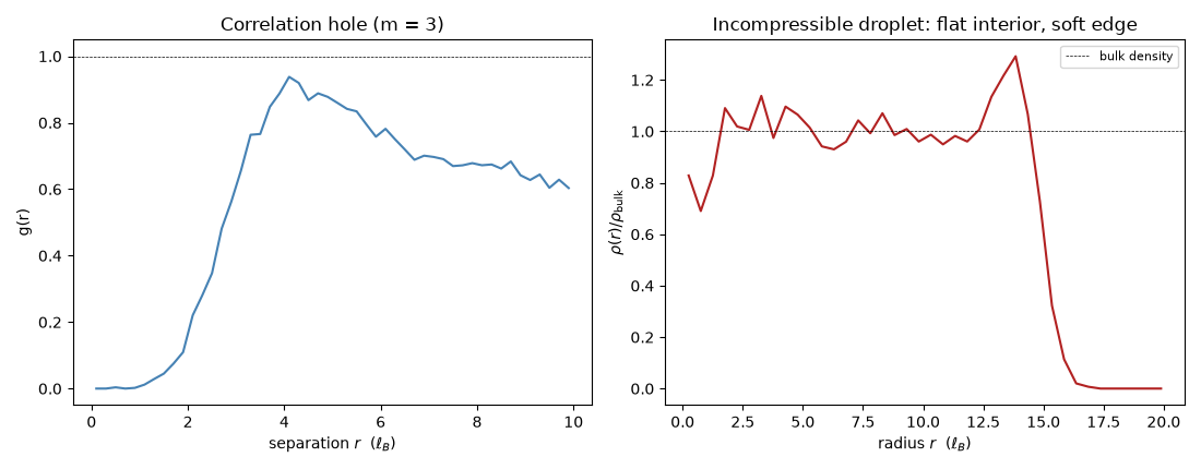
g(r) vanishes at zero separation and climbs to the uncorrelated value of 1 within a few magnetic lengths – particles are kept apart far more effectively than Pauli exclusion alone would manage, exactly the correlation the \((z_i-z_j)^m\) prefactor was built to enforce. The density profile is close to the exact bulk value \(\rho=1/(2\pi m\,\ell_B^2)\) through most of the droplet’s interior, falling off only within a few magnetic lengths of its edge – the real-space picture of the same incompressible liquid that makes the quantized Hall plateau itself possible.

plt.show()