Peierls Substitution: A Hofstadter-Like Spectrum from Landau’s Physics

Lev Landau showed that a charged particle in a uniform magnetic field has a kinetic-energy spectrum that collapses into discrete, macroscopically degenerate levels \(E_n = \hbar\omega_c(n + 1/2)\). On a lattice, the same continuum physics is reached through the Peierls substitution: each bond acquires a phase proportional to the flux threading the plaquettes it borders. apply_peierls_phase() implements exactly this, turning a uniform flux into a Hofstadter-like spectrum whose low-energy states bunch into near-degenerate groups – the lattice remnant of the continuum Landau tower.

import matplotlib.pyplot as plt
import numpy as np

from physicskit.condensed.tight_binding import apply_peierls_phase

A finite square patch threaded by uniform flux

One orbital per site on an L x L patch, nearest-neighbor hopping t=1 along both bonds of the square lattice.

L = 16
positions = np.array([[i, j] for i in range(L) for j in range(L)], dtype=float)
index = {(i, j): i * L + j for i in range(L) for j in range(L)}
bonds = []
for i in range(L):
    for j in range(L):
        if i + 1 < L:
            bonds.append((index[(i, j)], index[(i + 1, j)], 1.0))
        if j + 1 < L:
            bonds.append((index[(i, j)], index[(i, j + 1)], 1.0))

Peierls substitution and diagonalization

apply_peierls_phase multiplies each bond by the Landau-gauge phase set by the flux per plaquette; the resulting Hermitian hopping matrix is then diagonalized directly.

def _spectrum_at_flux(flux: float) -> np.ndarray:
    phased = apply_peierls_phase(positions, bonds, flux_quanta_per_plaquette=flux, area_per_plaquette=1.0)
    Hmat = np.zeros((L * L, L * L), dtype=complex)
    for i, j, amp in phased:
        Hmat[i, j] += amp
        Hmat[j, i] += np.conj(amp)
    return np.linalg.eigvalsh(Hmat)


flux = 1.0 / 8.0
energies = np.sort(_spectrum_at_flux(flux))

The lattice remnant of the Landau tower

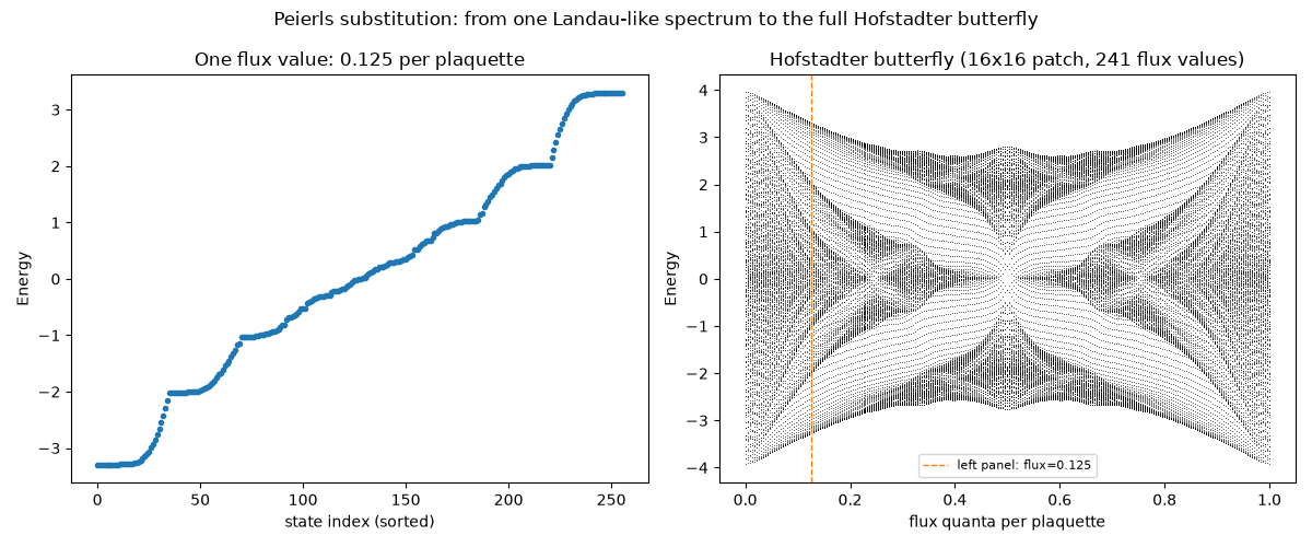
Instead of a smooth continuum, the low-energy spectrum bunches into near-degenerate groups separated by gaps – the finite-lattice, Peierls-substituted analogue of Landau’s equally spaced \(E_n\) levels.

The Hofstadter butterfly: every flux value at once

The single flux above is one vertical slice of a much richer object. Sweeping the flux per plaquette continuously from 0 to 1 and stacking every resulting spectrum produces the Hofstadter butterfly: the self-similar, fractal pattern of allowed energies that a charged particle on a lattice threaded by a magnetic field traces out, first predicted by Douglas Hofstadter (1976). This finite L x L patch cannot resolve the butterfly’s full fractal structure (that needs the exact Bloch (Harper) problem on the flux’s magnetic unit cell), but the same Peierls-substituted finite-lattice diagonalization used for one flux value above, repeated across the full flux range, already traces out its characteristic large-scale wings and gaps.

flux_values = np.linspace(0.0, 1.0, 241)
butterfly = np.array([_spectrum_at_flux(f) for f in flux_values])

fig, (ax1, ax2) = plt.subplots(1, 2, figsize=(12, 5))

ax1.plot(energies, "o", ms=3)
ax1.set_xlabel("state index (sorted)")
ax1.set_ylabel("Energy")
ax1.set_title(f"One flux value: {flux:.3f} per plaquette")

ax2.plot(np.tile(flux_values[:, None], (1, butterfly.shape[1])), butterfly, ",", color="black", alpha=0.6)
ax2.axvline(flux, color="C1", ls="--", lw=1, label=f"left panel: flux={flux:.3f}")
ax2.set_xlabel("flux quanta per plaquette")
ax2.set_ylabel("Energy")
ax2.set_title(f"Hofstadter butterfly ({L}x{L} patch, {len(flux_values)} flux values)")
ax2.legend(fontsize=8)

fig.suptitle("Peierls substitution: from one Landau-like spectrum to the full Hofstadter butterfly")
fig.tight_layout()

gaps = np.diff(energies[:40])
print(f"largest gaps among the lowest 40 states: {np.sort(gaps)[-4:]}")

largest gaps among the lowest 40 states: [0.1222108  0.13303268 0.13693357 0.14320934]