Schrodinger’s wavepacket spreading

Erwin Schrodinger’s 1926 wave equation,

\[i\hbar\partial_t\psi = -\frac{\hbar^2}{2m}\nabla^2\psi + V\psi,\]

made a radical and verifiable prediction: a localized particle’s wavefunction inevitably spreads out over time, even in free space (\(V=0\)). nls_evolve() solves the nonlinear Schrodinger equation \(i\partial_t\psi + \tfrac12\partial_x^2\psi + g|\psi|^2\psi = 0\) (natural units \(\hbar=m=1\)); switching its nonlinearity off (g=0) leaves exactly Schrodinger’s free-particle equation above. Starting from a Gaussian wavepacket of initial width \(\sigma_0\), this reproduces the free-particle spreading law

\[\sigma(t) = \sigma_0\sqrt{1+\left(\frac{t}{2\sigma_0^2}\right)^2}\]

directly from that solver.

import matplotlib.pyplot as plt
import numpy as np

from physicskit.fields import nls_evolve, nls_evolve_frames, plot_field_1d

A narrow Gaussian wavepacket, \(\sigma_0 = 2\) (units \(\hbar=m=1\))

N, L, sigma0 = 2048, 200.0, 2.0
x = np.linspace(-L / 2, L / 2, N, endpoint=False)
psi0 = np.exp(-(x**2) / (4 * sigma0**2)).astype(complex)
psi0 /= np.sqrt(np.sum(np.abs(psi0) ** 2) * (x[1] - x[0]))

Free-particle evolution: g=0 keeps only Schrodinger’s linear term

t_final, steps = 6.0, 3000
psi = nls_evolve(psi0, x, dt=t_final / steps, steps=steps, g=0.0)

The wavepacket spreads exactly as predicted by the free-particle spreading law.

dens = np.abs(psi) ** 2 / np.sum(np.abs(psi) ** 2 * (x[1] - x[0]))
sigma_num = np.sqrt(np.sum(x**2 * dens) * (x[1] - x[0]))
sigma_theory = sigma0 * np.sqrt(1 + (t_final / (2 * sigma0**2)) ** 2)

fig, ax = plot_field_1d(x, np.abs(psi0), label="t = 0")
plot_field_1d(x, np.abs(psi), ax=ax, label=f"t = {t_final}")
ax.set_title(f"sigma(t): numeric {sigma_num:.3f}, theory {sigma_theory:.3f}")
fig.tight_layout()

print(f"numeric sigma(t={t_final}) = {sigma_num:.4f}")
print(f"theory  sigma(t={t_final}) = {sigma_theory:.4f}  (sigma0 * sqrt(1+(t/2 sigma0^2)^2))")

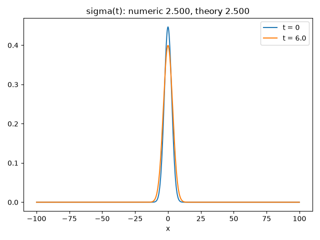
numeric sigma(t=6.0) = 2.5000
theory  sigma(t=6.0) = 2.5000  (sigma0 * sqrt(1+(t/2 sigma0^2)^2))

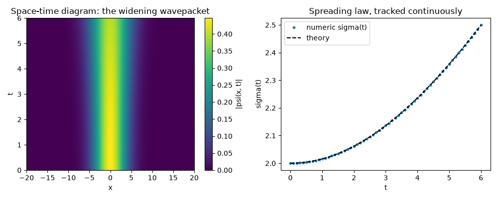
A space-time diagram, and sigma(t) tracked continuously against theory

The two-instant comparison above only checks \(\sigma(t)\) at the very end; recording every intermediate snapshot with nls_evolve_frames() (the same free-particle split-step integrator, restructured only to also keep a history) shows the whole spreading process at once, as a widening light-cone-like wedge in space and time, and lets \(\sigma(t)\) be measured from the recorded density at every frame, not just the last one – tracking the free-particle spreading law continuously rather than checking a single endpoint.

n_frames = 60
frames, times = nls_evolve_frames(psi0, x, dt=t_final / steps, steps_per_frame=steps // n_frames, n_frames=n_frames, g=0.0)
frame_dens = np.abs(frames) ** 2
frame_dens /= np.sum(frame_dens, axis=1, keepdims=True) * (x[1] - x[0])
sigma_num_t = np.sqrt(np.sum(x[np.newaxis, :] ** 2 * frame_dens, axis=1) * (x[1] - x[0]))
sigma_theory_t = sigma0 * np.sqrt(1 + (times / (2 * sigma0**2)) ** 2)

fig2, (ax_space, ax_sigma) = plt.subplots(1, 2, figsize=(10, 4))
extent = (x.min(), x.max(), times.min(), times.max())
im = ax_space.imshow(np.abs(frames), extent=extent, origin="lower", aspect="auto", cmap="viridis")
fig2.colorbar(im, ax=ax_space, label="|psi(x, t)|")
ax_space.set_xlim(-8 * sigma_theory_t[-1], 8 * sigma_theory_t[-1])
ax_space.set_xlabel("x")
ax_space.set_ylabel("t")
ax_space.set_title("Space-time diagram: the widening wavepacket")

ax_sigma.plot(times, sigma_num_t, "o", markersize=3, label="numeric sigma(t)")
ax_sigma.plot(times, sigma_theory_t, "k--", label="theory")
ax_sigma.set_xlabel("t")
ax_sigma.set_ylabel("sigma(t)")
ax_sigma.set_title("Spreading law, tracked continuously")
ax_sigma.legend()
fig2.tight_layout()