An exact kink-antikink collision from inverse scattering

Gardner, Greene, Kruskal, and Miura’s 1967 inverse scattering transform (IST) explained why solitons collide elastically, and showed that KdV was only the first of a broad class of exactly integrable equations – the Sine-Gordon equation

\[\partial_t^2 u - \partial_x^2 u + \sin u = 0\]

included. For Sine-Gordon, the technique yields a closed-form two-soliton solution directly, without any numerical time-stepping,

\[u(x,t) = 4\arctan\!\left(\frac{\sinh(\gamma v t)}{v\,\cosh(\gamma x)}\right), \qquad \gamma = \frac{1}{\sqrt{1-v^2}},\]

describing a kink and an antikink, each moving at speed \(v\) toward \(x=0\), that approach, collide, and pass through each other exactly. This integrates that same closed-form initial condition (well before the collision, at \(t=T_0 \ll 0\)) forward numerically with sine_gordon_evolve(), entirely independently of the exact solution, and checks the two agree at the corresponding time after the collision.

import matplotlib.pyplot as plt
import numpy as np

from physicskit.fields import plot_field_1d, sine_gordon_evolve, sine_gordon_evolve_frames


def sg_kink_antikink(x, t, v):
    """The IST-derived closed-form kink-antikink solution of u_tt - u_xx + sin(u) = 0."""
    gamma = 1.0 / np.sqrt(1 - v**2)
    return 4 * np.arctan(np.sinh(gamma * v * t) / (v * np.cosh(gamma * x)))

The exact IST kink-antikink collision solution, well before the collision

N, L, v, T0 = 4000, 200.0, 0.5, -40.0
x = np.linspace(-L / 2, L / 2, N)
dx = x[1] - x[0]
dt = 0.4 * dx
u_prev = sg_kink_antikink(x, T0 - dt, v)
u0 = sg_kink_antikink(x, T0, v)

Integrate this closed-form initial condition numerically through the collision, entirely independently of the exact IST solution ————————————————————————–

steps = int(round((2 * abs(T0)) / dt))
u, _ = sine_gordon_evolve(u0, u_prev, x, dt, steps)

The two solitons pass straight through each other, exactly as the closed-form IST solution (evaluated at the same final time) predicts – the deeper mathematical structure behind the elastic collisions.

expected = sg_kink_antikink(x, T0 + steps * dt, v)
max_dev = np.max(np.abs(u - expected))

fig, ax = plot_field_1d(x, u0, label="t = T0 (approaching)")
plot_field_1d(x, u, ax=ax, label="t = -T0 (departed)")
ax.set_title(f"max deviation from exact IST solution: {max_dev:.2e}")
fig.tight_layout()

print(f"max deviation of the numerical evolution from the exact IST solution: {max_dev:.2e}")

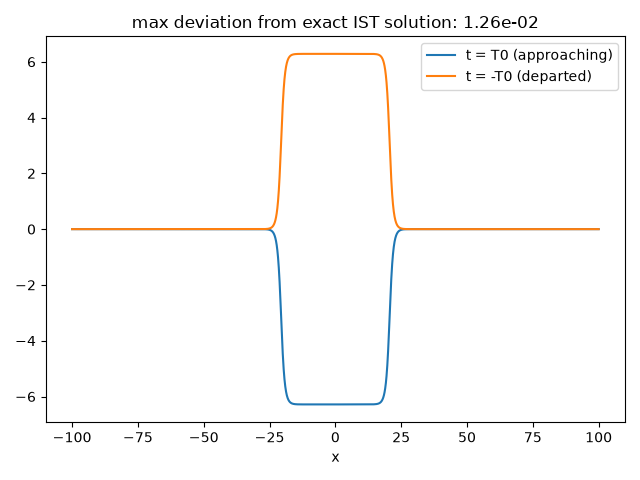
max deviation of the numerical evolution from the exact IST solution: 1.26e-02

A space-time diagram of the collision itself

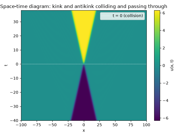
The before/after comparison above only checks the two endpoints; re-running the same leapfrog integration with sine_gordon_evolve_frames() (identical physics, restructured only to also keep a history) and stacking the recorded snapshots into an image shows the actual collision: a kink and an antikink, each a fixed \(2\pi\)-twist ridge, approaching from opposite directions, merging briefly near \(x=0\), and separating again afterward with each ridge’s slope unchanged – the IST solution’s “pass through each other exactly” made visible frame by frame.

n_frames = 100
steps_per_frame = max(steps // n_frames, 1)
frames, snap_times = sine_gordon_evolve_frames(u0, u_prev, x, dt, steps_per_frame=steps_per_frame, n_frames=n_frames)

fig2, ax2 = plt.subplots()
extent = (x.min(), x.max(), T0, T0 + snap_times[-1])
im = ax2.imshow(frames, extent=extent, origin="lower", aspect="auto", cmap="viridis")
fig2.colorbar(im, ax=ax2, label="u(x, t)")
ax2.axhline(0.0, color="w", ls=":", lw=1, label="t = 0 (collision)")
ax2.set_xlabel("x")
ax2.set_ylabel("t")
ax2.set_title("Space-time diagram: kink and antikink colliding and passing through")
ax2.legend(loc="upper right")
fig2.tight_layout()