Gauss’s ABCD formalism: a composite system as a matrix product

Carl Friedrich Gauss showed that any centered optical system, however many lenses and refracting surfaces it contains, can be fully characterized in the paraxial approximation by linear algebra rather than surface-by-surface trigonometry: every elementary optical element is a linear map on the ray state \((y, \theta)\) – height above the axis and angle to it –

\[\begin{split}\begin{pmatrix} y_{\text{out}} \\ \theta_{\text{out}} \end{pmatrix} = \begin{pmatrix} A & B \\ C & D \end{pmatrix} \begin{pmatrix} y_{\text{in}} \\ \theta_{\text{in}} \end{pmatrix},\end{split}\]

and a compound system’s matrix is simply the ordered product of its elements’ matrices, \(M = M_n \cdots M_2 M_1\) (rightmost applied first). Every function in physicskit.optics.ray – free_space(), thin_lens(), and the rest – returns one elementary Gauss/ABCD matrix, and system_matrix() multiplies them in traversal order, exactly Gauss’s composition rule. Below, a simple imaging system – free-space propagation, a thin lens, then more free-space propagation – is built two ways: once by composing system_matrix() from named elements, and once by directly multiplying the three elementary matrices by hand, to confirm they agree exactly.

import matplotlib.pyplot as plt
import numpy as np

from physicskit.optics.ray import OpticalElement, OpticalSystem, free_space, thin_lens
from physicskit.optics.visualizers import plot_ray_trace

A simple imaging system: object distance, thin lens, image distance

d1, f, d2 = 0.3, 0.1, 0.15
system = OpticalSystem(
    [
        OpticalElement(free_space(d1), name="object -> lens", length=d1),
        OpticalElement(thin_lens(f), name="lens"),
        OpticalElement(free_space(d2), name="lens -> image", length=d2),
    ]
)

Gauss’s composition rule: the whole system is just matrix multiplication. Building the system matrix by hand, as an explicit product of the three element matrices, must agree exactly with system_matrix().

M_direct = free_space(d2) @ thin_lens(f) @ free_space(d1)
M_system = system.system_matrix()
matrices_agree = np.allclose(M_direct, M_system)

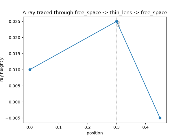
fig, ax = plot_ray_trace(system, y0=0.01, theta0=0.05)
ax.set_title("A ray traced through free_space -> thin_lens -> free_space")

print("hand-built product M = free_space(d2) @ thin_lens(f) @ free_space(d1):")
print(M_direct)
print("\nOpticalSystem.system_matrix() (elements multiplied in traversal order):")
print(M_system)
print(f"\nmatrices agree: {matrices_agree}")

trajectory = system.trace_ray(y0=0.01, theta0=0.05)
print(f"\nray height/angle at each plane:\n{trajectory}")

hand-built product M = free_space(d2) @ thin_lens(f) @ free_space(d1):
[[-5.00000000e-01  2.77555756e-17]
 [-1.00000000e+01 -2.00000000e+00]]

OpticalSystem.system_matrix() (elements multiplied in traversal order):
[[ -0.5   0. ]
 [-10.   -2. ]]

matrices agree: True

ray height/angle at each plane:
[[ 0.01   0.05 ]
 [ 0.025  0.05 ]
 [ 0.025 -0.2  ]
 [-0.005 -0.2  ]]

A ray fan: imaging, not just tracing, one ray

A single traced ray only shows what the ABCD matrix does to one input state. Tracing a fan of rays launched from the same off-axis object point y0 but at many different angles theta0 – each just another call to trace_ray() through the very same system – shows the imaging property that composed ABCD matrix actually encodes: since d2 here was chosen to satisfy the thin lens conjugate relation for d1 and f, every ray of the fan, however steep, is bent by the lens so as to reconverge at the same height at the image plane.

object_height = 0.01
angles = np.linspace(-0.08, 0.08, 9)
positions = np.concatenate(([0.0], np.cumsum([el.length for el in system.elements])))

fig2, ax2 = plt.subplots(figsize=(7, 3.5))
for theta0 in angles:
    fan_trajectory = system.trace_ray(y0=object_height, theta0=theta0)
    ax2.plot(positions, fan_trajectory[:, 0], color="C0", alpha=0.7)
image_heights = np.array([system.trace_ray(y0=object_height, theta0=th)[-1, 0] for th in angles])
ax2.axvline(positions[-1], color="r", ls="--", lw=1, label="image plane")
ax2.axhline(0.0, color="k", lw=0.5)
ax2.set_xlabel("position")
ax2.set_ylabel("ray height y")
ax2.legend(fontsize=8)
ax2.set_title(f"Ray fan from one object point: all {len(angles)} rays reconverge at the image plane")
fig2.tight_layout()

print(f"\nray-fan image heights at the final plane (should all coincide): {image_heights}")
print(f"spread of image heights across the fan: {image_heights.max() - image_heights.min():.2e}")

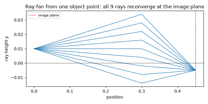
ray-fan image heights at the final plane (should all coincide): [-0.005 -0.005 -0.005 -0.005 -0.005 -0.005 -0.005 -0.005 -0.005]
spread of image heights across the fan: 3.47e-18