Two-mirror resonator stability (Maiman’s ruby laser cavity)

Theodore Maiman’s 1960 ruby laser used a resonator formed by two mirrors bounding an amplifying medium – precisely the kind of optical cavity that ray-transfer matrix theory was soon developed to analyze. This package does not model laser gain media, but spherical_mirror() and cavity_round_trip_matrix() build the ABCD round-trip matrix of a two-mirror resonator like Maiman’s, and cavity_stability() tests whether such a cavity traps light indefinitely (a stable resonator, \(|A+D| \le 2\)) or walks rays out of the cavity on successive round trips.

import matplotlib.pyplot as plt
import numpy as np

from physicskit.optics.ray import (
    OpticalElement,
    cavity_round_trip_matrix,
    cavity_stability,
    free_space,
    spherical_mirror,
)

Scan the mirror separation of a symmetric two-mirror cavity

R1, R2 = 2.0, 2.0  # mirror radii of curvature (m)
lengths = np.linspace(0.01, 4.5, 400)  # cavity lengths to scan (m)

stable = []
for d in lengths:
    M = cavity_round_trip_matrix(
        [
            OpticalElement(spherical_mirror(R1), name="M1"),
            OpticalElement(free_space(d), name="gap"),
            OpticalElement(spherical_mirror(R2), name="M2"),
            OpticalElement(free_space(d), name="gap"),
        ]
    )
    stable.append(cavity_stability(M))
stable = np.array(stable)

For a symmetric confocal-type cavity, the g-parameter product \(g_1 g_2 = (1 - d/R)^2\) crosses the stability boundary \(g_1g_2 = 1\) exactly at \(d = 2R\); the boundary found directly from the ABCD round-trip matrix should land at exactly that point.

fig, ax = plt.subplots(figsize=(7, 3))
ax.plot(lengths, stable, drawstyle="steps-post")
ax.axvline(2 * R1, color="r", ls="--", label="d = 2R (predicted stability edge)")
ax.set_xlabel("cavity length d (m)")
ax.set_ylabel("is_stable")
ax.legend()
ax.set_title(f"Two-mirror resonator (R1=R2={R1} m): stable only for d < 2R")
fig.tight_layout()

boundary_index = np.argmax(~stable)
print(f"mirror radii R1 = R2 = {R1} m; predicted stability edge at d = 2R = {2 * R1} m")
print(f"numerically found: cavity stable for the first {boundary_index} of {len(lengths)} scanned lengths")
print(f"transition occurs between d = {lengths[boundary_index - 1]:.4f} m and d = {lengths[boundary_index]:.4f} m")

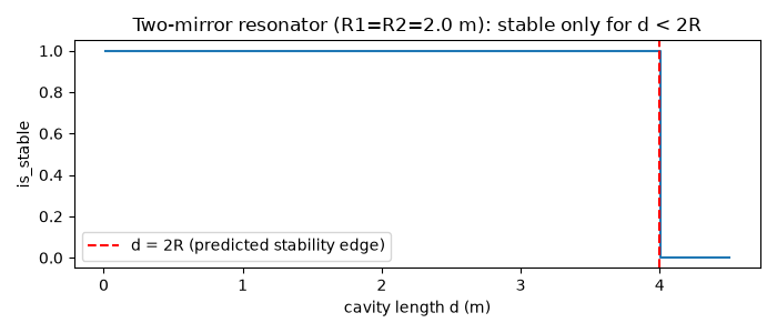
mirror radii R1 = R2 = 2.0 m; predicted stability edge at d = 2R = 4.0 m
numerically found: cavity stable for the first 355 of 400 scanned lengths
transition occurs between d = 3.9936 m and d = 4.0049 m

The classic two-parameter stability diagram

Scanning only the cavity length at fixed mirror radii, as above, cuts through just one line of the textbook resonator stability diagram. The full diagram sweeps two cavity parameters at once – here the cavity length d and the second mirror’s radius of curvature R2 (R1 held fixed) – and asks cavity_stability() at every point of the grid, tracing out the stable/unstable regions (in the reduced g-parameter variables \(g_i = 1 - d/R_i\), the familiar hyperbolic stability wedge bounded by \(g_1 g_2 = 0\) and \(g_1 g_2 = 1\)).

R2_values = np.linspace(0.3, 4.5, 250)
d_values = np.linspace(0.01, 4.5, 250)
stability_map = np.zeros((len(R2_values), len(d_values)), dtype=bool)
for i, R2_i in enumerate(R2_values):
    for j, d_j in enumerate(d_values):
        M_ij = cavity_round_trip_matrix(
            [
                OpticalElement(spherical_mirror(R1), name="M1"),
                OpticalElement(free_space(d_j), name="gap"),
                OpticalElement(spherical_mirror(R2_i), name="M2"),
                OpticalElement(free_space(d_j), name="gap"),
            ]
        )
        stability_map[i, j] = cavity_stability(M_ij)

fig2, ax2 = plt.subplots(figsize=(6.5, 5))
im = ax2.pcolormesh(d_values, R2_values, stability_map, shading="auto", cmap="Greens", vmin=0, vmax=1.3)
ax2.plot(lengths, np.full_like(lengths, R2), "r--", lw=1, label=f"1D scan above (R2={R2} m)")
ax2.set_xlabel("cavity length d (m)")
ax2.set_ylabel("mirror radius R2 (m)")
ax2.legend(fontsize=8)
ax2.set_title(f"Stability phase diagram (R1={R1} m fixed): green = stable resonator")
fig2.tight_layout()

fraction_stable = stability_map.mean()
print(f"\nfull (d, R2) stability map: {fraction_stable * 100:.1f}% of the scanned grid is a stable resonator")

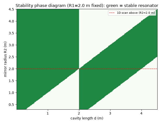
full (d, R2) stability map: 62.8% of the scanned grid is a stable resonator