From collision to detector: a hard scatter, its shower, and its tracks

A real collider event unfolds in three stages, each with its own physics: a hard 2-to-2 collision fixes the initial parton kinematics from exact relativistic two-body phase space; each outgoing parton then radiates repeatedly (a “shower”) until its energy falls below a hadronization scale, producing a collimated spray of partons – a jet; and finally every final-state charged particle curves through the detector’s magnetic field, \(r = p_T/(qB)\), while neutral particles fly straight, both depositing their energy once they reach the calorimeter.

\[e^+ e^- \to q\bar q \ (\sqrt{s} \text{ fixed}) \ \longrightarrow\ \text{parton shower} \ \longrightarrow\ \text{jets} \ \longrightarrow\ \text{curved tracks in } B.\]

This example chains exactly these three stages using nothing but the building blocks already validated elsewhere in physicskit.particle: two_body_decay() for the hard vertex, parton_shower() for the cascade, and charged_track_points() (via animate_detector_event()) for the detector response.

import numpy as np

from physicskit.particle.collider import cluster_into_jets, parton_shower, shower_leaves
from physicskit.particle.decays import two_body_decay
from physicskit.particle.visualizers import animate_detector_event, animate_parton_shower

rng = np.random.default_rng(0)

Stage 1: the hard collision, e+e- -> q qbar

Exact two-body phase space at a chosen center-of-mass energy fixes the outgoing quark and antiquark’s four-momenta – back to back, each carrying half of sqrt(s) – exactly the same kinematic building block used throughout physicskit.particle for two-body decays and resonance production.

sqrt_s = 90.0  # GeV-like units, e.g. roughly a Z-pole collision
m_q = 0.0
cos_theta = float(rng.uniform(-1.0, 1.0))
phi = float(rng.uniform(0.0, 2.0 * np.pi))
p_quark, p_antiquark = two_body_decay(sqrt_s, m_q, m_q, cos_theta, phi)
print(f"sqrt(s) = {sqrt_s:.1f}, quark E = {p_quark.E:.2f}, antiquark E = {p_antiquark.E:.2f}")
print(f"back-to-back check: |p_quark + p_antiquark| (3-mom.) = {np.linalg.norm(p_quark.p_vec + p_antiquark.p_vec):.2e}")

sqrt(s) = 90.0, quark E = 45.00, antiquark E = 45.00
back-to-back check: |p_quark + p_antiquark| (3-mom.) = 0.00e+00

Stage 2: each parton showers into a jet

The quark-side shower alone already shows the full “collision -> shower -> jets” story: a single energetic quark radiates repeatedly, its products increasingly collimated by the boost back to the lab frame, until cluster_into_jets() recovers the (here, single) jet axis animate_parton_shower overlays automatically.

root_q = parton_shower(p_quark.E, flavor0="q", rng=np.random.default_rng(1))
anim_shower = animate_parton_shower(root_q, n_jets=1)

import matplotlib.pyplot as plt  # noqa: E402

plt.show()

To save the shower animation to a file instead of (or in addition to) displaying it interactively, use e.g.:

anim_shower.save("parton_shower.gif", writer="pillow", fps=8)

Beyond one shower: multiplicity and quark/gluon composition fluctuations

The animation above is a single draw from a genuinely stochastic branching process. Re-running parton_shower() many times at the same initial quark energy (only the random splitting angles and the random g -> gg vs. g -> q qbar choice at each gluon node differ) turns that one event into the kind of statistical ensemble real jet-multiplicity and quark/gluon-composition measurements characterize – a distribution, not a single number.

n_showers = 400
multiplicities = np.empty(n_showers, dtype=int)
gluon_fractions = np.empty(n_showers)
for i in range(n_showers):
    root_i = parton_shower(p_quark.E, flavor0="q", rng=np.random.default_rng(1000 + i))
    leaves_i = shower_leaves(root_i)
    multiplicities[i] = len(leaves_i)
    gluon_fractions[i] = np.mean([leaf.flavor == "g" for leaf in leaves_i])

fig, (ax_mult, ax_flav) = plt.subplots(1, 2, figsize=(10, 4))

ax_mult.hist(multiplicities, bins=np.arange(multiplicities.min(), multiplicities.max() + 2) - 0.5, color="C0", edgecolor="white")
ax_mult.axvline(len(shower_leaves(root_q)), color="C3", ls="--", label="animated event above")
ax_mult.set_xlabel("final-state particles per shower")
ax_mult.set_ylabel("showers")
ax_mult.set_title(f"jet multiplicity ({n_showers} independent showers)")
ax_mult.legend()

ax_flav.hist(gluon_fractions, bins=30, color="C1", edgecolor="white")
ax_flav.set_xlabel("gluon fraction of final-state partons")
ax_flav.set_ylabel("showers")
ax_flav.set_title("quark/gluon composition")

fig.suptitle("Shower-to-shower fluctuations at fixed initial quark energy")
fig.tight_layout()
plt.show()

print(f"multiplicity across {n_showers} showers: mean={multiplicities.mean():.1f}, std={multiplicities.std():.1f}")
print(f"gluon fraction: mean={gluon_fractions.mean():.3f}, std={gluon_fractions.std():.3f}")

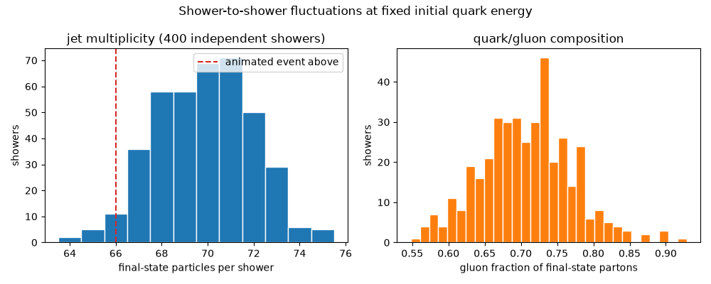
multiplicity across 400 showers: mean=69.9, std=2.1
gluon fraction: mean=0.709, std=0.063

Stage 3: final-state particles reach the detector

The shower’s leaves – its stable, non-branching final state – are handed to a schematic detector: alternating charges for illustration (a real fragmentation model would assign hadron charges by flavor), curving in a uniform axial field exactly as charged_track_points() prescribes.

leaves = shower_leaves(root_q)
jets = cluster_into_jets(leaves, n_jets=1)
print(f"final-state particles: {len(leaves)}, clustered into {len(jets)} jet(s)")

four_vectors = [leaf.four_vector for leaf in leaves]
charges = [1.0 if i % 2 == 0 else -1.0 for i in range(len(leaves))]
anim_detector = animate_detector_event(four_vectors, charges, B=0.15, n_frames=50)
plt.show()

final-state particles: 66, clustered into 1 jet(s)

To save the detector animation to a file instead of (or in addition to) displaying it interactively, use e.g.:

anim_detector.save("detector_event.gif", writer="pillow", fps=10)