Anderson, Neddermeyer, Street, and Stevenson: discovery of the muon

By 1936 cosmic-ray tracks fell into two groups. Some particles showered in lead, like electrons. Others went straight through thick lead losing only ionization energy. If those penetrating particles were electrons, bremsstrahlung should have stopped them; if they were protons, they should have ionized far more heavily at their momentum. Anderson and Neddermeyer (1937) concluded they had intermediate mass. Street and Stevenson (1937) measured one track’s curvature and ionization density together and got about 130 electron masses (modern: 206.8).

A cloud chamber gives two independent numbers per track: momentum from the curvature in the magnetic field, and speed from the ionization density, which by the Bethe formula depends only on \(\beta\gamma = p/(mc)\). Together they fix the mass. This example draws tracks of equal momentum with charged_track_points(), inverts the Bethe formula for simulated measurements, and compares radiative energy loss in lead for electrons and muons.

import matplotlib.pyplot as plt
import numpy as np
from scipy.optimize import brentq

from physicskit.particle.collider import charged_track_points
from physicskit.particle.kinematics import FourVector

masses = {"electron": 0.511, "muon": 105.66, "proton": 938.27}  # MeV
colors = {"electron": "steelblue", "muon": "darkorange", "proton": "firebrick"}


def bethe(betagamma, I=85.7e-6, ZA=0.499):
    """Mean ionization loss in air [MeV cm^2/g], unit charge.

    No density-effect correction: fine for a gas below the Fermi plateau,
    and a rough guide for the electron's relativistic rise.
    """
    m_e, K = 0.511, 0.307075
    bg2 = betagamma**2
    b2 = bg2 / (1 + bg2)
    Tmax = 2 * m_e * bg2  # heavy-particle approximation
    return K * ZA / b2 * (0.5 * np.log(2 * m_e * bg2 * Tmax / I**2) - b2)


bg_min = brentq(lambda x: np.gradient(bethe(np.array([x * 0.999, x, x * 1.001])))[1], 1.0, 10.0)
dEdx_min = bethe(bg_min)

Same momentum, same curvature

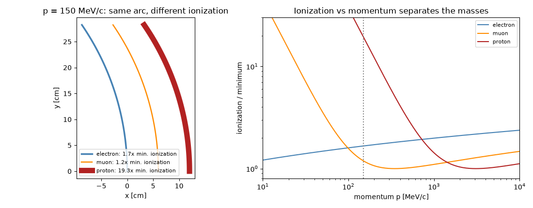
At 150 MeV/c in a 1 T field all three bend identically. Curvature alone can’t tell them apart (tracks shifted sideways for clarity; line width shows ionization density).

p = 150.0
fig1, (ax1, ax2) = plt.subplots(1, 2, figsize=(11, 4.3))
for offset, (name, m) in enumerate(masses.items()):
    fv = FourVector(np.hypot(p, m), 0.0, p / 1e3, 0.0)
    pts = charged_track_points(fv, charge=-1.0, B=0.3, vertex=(0.06 * offset, 0.0), path_length=0.3)
    ionization = bethe(p / m) / dEdx_min
    ax1.plot(pts[:, 0] * 100, pts[:, 1] * 100, color=colors[name], lw=min(1.5 * ionization, 8), label=f"{name}: {ionization:.1f}x min. ionization")
ax1.set_aspect("equal")
ax1.set_xlabel("x [cm]")
ax1.set_ylabel("y [cm]")
ax1.set_title(f"p = {p:.0f} MeV/c: same arc, different ionization")
ax1.legend(fontsize=8)

bg = np.geomspace(0.1, 1e5, 500)
for name, m in masses.items():
    pp = bg * m
    ax2.loglog(pp, bethe(bg) / dEdx_min, color=colors[name], label=name)
ax2.axvline(p, color="0.5", ls=":")
ax2.set_xlim(10, 1e4)
ax2.set_ylim(0.8, 30)
ax2.set_xlabel("momentum p [MeV/c]")
ax2.set_ylabel("ionization / minimum")
ax2.set_title("Ionization vs momentum separates the masses")
ax2.legend(fontsize=8)
fig1.tight_layout()

Measuring the mass

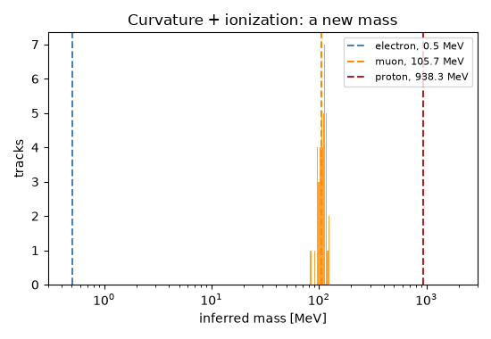
Fifty simulated penetrating tracks: momentum from curvature (5% resolution) and ionization from droplet counting (10%). Invert the Bethe curve on its low-velocity branch for \(\beta\gamma\), then \(m = p/(\beta\gamma)\).

rng = np.random.default_rng(1937)
p_true = rng.uniform(40, 90, 50)
bg_true = p_true / masses["muon"]
p_meas = p_true * (1 + 0.05 * rng.standard_normal(50))
ion_meas = bethe(bg_true) / dEdx_min * (1 + 0.10 * rng.standard_normal(50))
bg_fit = np.array([brentq(lambda x, y=y: bethe(x) / dEdx_min - y, 0.05, bg_min) for y in ion_meas])
m_fit = p_meas / bg_fit
print(f"inferred mass: {np.median(m_fit):.0f} MeV  ({np.median(m_fit) / masses['electron']:.0f} electron masses; muon: 207)")
print(f"spread (16-84%): {np.percentile(m_fit, 16):.0f} - {np.percentile(m_fit, 84):.0f} MeV")

inferred mass: 108 MeV  (211 electron masses; muon: 207)
spread (16-84%): 99 - 116 MeV

Why it penetrates lead

Bremsstrahlung scales as \(1/m^2\), so a muon’s radiation length is \((m_\mu/m_e)^2\approx43{,}000\) times an electron’s. Through 1 cm of lead (\(X_0=0.56\) cm) a 300 MeV electron keeps \(e^{-x/X_0}\) of its energy on average; a muon loses only about 13 MeV to ionization.

X0_Pb, x = 0.56, 1.0
E0 = 300.0
E_e = E0 * np.exp(-x / X0_Pb)
E_mu = E0 - 12.7 * x - E0 * (1 - np.exp(-x / (X0_Pb * (masses["muon"] / masses["electron"]) ** 2)))
print(f"\nafter 1 cm of lead: electron {E_e:.0f} MeV, muon {E_mu:.0f} MeV  (starting at {E0:.0f} MeV)")

fig2, ax3 = plt.subplots(figsize=(5.5, 3.8))
ax3.hist(m_fit, bins=20, color="darkorange", alpha=0.8)
for name, m in masses.items():
    ax3.axvline(m, color=colors[name], ls="--", label=f"{name}, {m:.1f} MeV")
ax3.set_xscale("log")
ax3.set_xlim(0.3, 3000)
ax3.set_xlabel("inferred mass [MeV]")
ax3.set_ylabel("tracks")
ax3.set_title("Curvature + ionization: a new mass")
ax3.legend(fontsize=8)
fig2.tight_layout()

plt.show()

after 1 cm of lead: electron 50 MeV, muon 287 MeV  (starting at 300 MeV)

Check

Curvature (momentum) plus ionization (beta gamma) give the mass: ~207 electron masses; and a muon, unlike an electron, does not shower in lead.

assert abs(np.median(m_fit) / masses["muon"] - 1) < 0.05
assert E_mu > 0.9 * E0 and E_e < 0.2 * E0
assert 3.0 < bg_min < 4.0