The radioactive decay law: Becquerel, Rutherford, and Soddy

Becquerel’s 1896 chance discovery – a uranium salt spontaneously exposing a photographic plate with no external excitation – opened radioactivity as a field; Rutherford and Soddy (1902-1903) showed the underlying law is a simple exponential,

\[N(t) = N_0\,e^{-\lambda t}, \qquad t_{1/2} = \frac{\ln2}{\lambda},\]

with decay constant \(\lambda\) characteristic of the parent species alone. This example builds that law directly from decay_constant(), radioactive_decay_number(), and activity() – exactly the blackening rate that exposed Becquerel’s plate – and checks the defining property of a half-life: the population halves in every successive interval of length \(t_{1/2}\), regardless of how much has already decayed.

import matplotlib.pyplot as plt
import numpy as np

from physicskit.particle.decays import (
    activity,
    decay_constant,
    half_life,
    radioactive_decay_number,
)

From half-life to decay constant, and back

A radium-226-like half-life, in days, for concreteness.

t_half = 1600.0 * 365.25  # ~1600 years, in days
lam = decay_constant(t_half)
print(f"half-life:     {t_half:.3f} days")
print(f"decay constant: {lam:.3e} / day")
print(f"round trip:    half_life(decay_constant(t_half)) = {half_life(lam):.3f} days (should equal t_half)")

half-life:     584400.000 days
decay constant: 1.186e-06 / day
round trip:    half_life(decay_constant(t_half)) = 584400.000 days (should equal t_half)

The exponential decay law

N0 = 1.0e6
t = np.linspace(0.0, 5.0 * t_half, 500)
N = radioactive_decay_number(N0, lam, t)
A = activity(N, lam)

fig, (ax1, ax2) = plt.subplots(1, 2, figsize=(11, 4.2))
ax1.plot(t / t_half, N, color="steelblue")
for k in range(1, 5):
    ax1.axvline(k, color="0.75", lw=0.8, ls="--")
ax1.set_xlabel(r"$t / t_{1/2}$")
ax1.set_ylabel("N(t)")
ax1.set_title("Exponential decay: halves every $t_{1/2}$")

ax2.semilogy(t / t_half, N, color="firebrick")
ax2.set_xlabel(r"$t / t_{1/2}$")
ax2.set_ylabel("N(t) (log scale)")
ax2.set_title("A straight line on a log axis -- the signature of exponential decay")
fig.tight_layout()

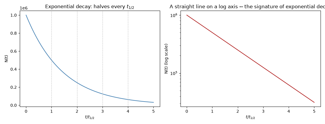
The defining property: halving in every interval of length t_1/2

Not just from t=0 – from any starting point. This is what makes a half-life a property of the isotope alone, independent of how much of the original sample remains, or when it was prepared.

for start_multiple in [0, 1, 2, 3]:
    t_start = start_multiple * t_half
    N_start = radioactive_decay_number(N0, lam, t_start)
    N_after_one_halflife = radioactive_decay_number(N0, lam, t_start + t_half)
    ratio = N_after_one_halflife / N_start
    print(f"N({start_multiple}*t_1/2) = {N_start:.4e}  ->  N({start_multiple + 1}*t_1/2) = {N_after_one_halflife:.4e}  (ratio = {ratio:.6f})")

print(f"\nactivity (Becquerel's actual observable, the plate-blackening rate) at t=0: {A[0]:.4e} decays/day")
print(f"activity after one half-life:                                            {activity(radioactive_decay_number(N0, lam, t_half), lam):.4e} decays/day")

plt.show()

N(0*t_1/2) = 1.0000e+06  ->  N(1*t_1/2) = 5.0000e+05  (ratio = 0.500000)
N(1*t_1/2) = 5.0000e+05  ->  N(2*t_1/2) = 2.5000e+05  (ratio = 0.500000)
N(2*t_1/2) = 2.5000e+05  ->  N(3*t_1/2) = 1.2500e+05  (ratio = 0.500000)
N(3*t_1/2) = 1.2500e+05  ->  N(4*t_1/2) = 6.2500e+04  (ratio = 0.500000)

activity (Becquerel's actual observable, the plate-blackening rate) at t=0: 1.1861e+00 decays/day
activity after one half-life:                                            5.9304e-01 decays/day