Plasma wakefield acceleration: a test charge surfing a traveling wave

Toshiki Tajima and John Dawson (1979) proposed firing an intense, short laser pulse into a plasma to excite a large-amplitude plasma wave in its wake, then injecting electrons to “surf” that wake’s electric field. Because a plasma wave’s field is not limited by material breakdown the way a copper accelerating cavity’s is, the resulting accelerating gradient can exceed conventional radio-frequency accelerators’ by three to four orders of magnitude – the proposal that launched the field of laser and beam-driven plasma wakefield acceleration.

Rather than deriving the wake self-consistently from a driver beam or laser pulse, this example prescribes it directly as a rigid traveling longitudinal electric-field wave of peak amplitude \(E_0\), wavenumber \(k\), and phase velocity \(v_{ph}\),

\[E_z(x, t) = E_0\cos\!\big[k(x - v_{ph}t)\big],\]

and injects a single test charge of charge \(q\) and mass \(m\) into it, integrating the Lorentz force with no magnetic field,

\[m\dot{\mathbf{v}} = q\,\mathbf{E}, \qquad \mathbf{E}=(E_z(x,t), 0, 0),\]

via boris_push(). A particle riding within one quarter-wavelength of the field’s zero-crossing near \(v\approx v_{ph}\) (the accelerating “bucket”) feels a sign-definite field and gains kinetic energy at the expense of the externally prescribed, infinite-energy-reservoir wave.

wakefield_e_field() evaluates \(E_z(x,t)\) directly, and simulate_wakefield_acceleration() injects the test charge into it with the same energy-conserving boris_push() used for gyro-orbits elsewhere in this package.

import matplotlib.pyplot as plt
import numpy as np

import physicskit as pk

A test electron launched near the wake’s own phase velocity

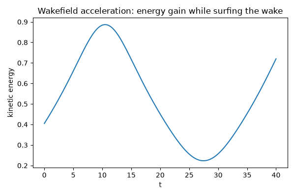
Riding the accelerating quarter-wave (“the bucket”) for as long as it stays trapped there, the particle gains kinetic energy at the expense of the (externally prescribed) wave.

result = pk.plasma.simulate_wakefield_acceleration(x0=0.0, v0=0.9, q=1.0, m=1.0, E0=0.05, k=1.0, v_phase=1.0, dt=0.01, steps=4000)

t, ke = result["t"], result["kinetic_energy"]
fig, ax = plt.subplots(figsize=(6, 4))
ax.plot(t, ke)
ax.set_xlabel("t")
ax.set_ylabel("kinetic energy")
ax.set_title("Wakefield acceleration: energy gain while surfing the wake")
fig.tight_layout()

plt.show()

Trapping in phase space: co-moving position vs. velocity

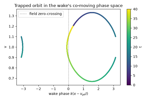
The energy trace above is a shadow of a richer, two-dimensional trapping picture. Reusing the same (x, v) history already returned by simulate_wakefield_acceleration(), plotting velocity against position in the wake’s own co-moving phase \(k(x - v_{ph}t)\) shows the particle orbiting a fixed point near \(v\approx v_{ph}\) instead of drifting through phase indefinitely – the phase-space signature of a particle trapped in the accelerating bucket rather than merely accelerated once and released.

x, v = result["x"], result["v"]
phase = np.mod(1.0 * (x - 1.0 * t) + np.pi, 2 * np.pi) - np.pi

fig, ax = plt.subplots(figsize=(6, 4))
sc = ax.scatter(phase, v, c=t, cmap="viridis", s=4)
fig.colorbar(sc, ax=ax, label="t")
ax.axvline(0.0, color="gray", linestyle="--", linewidth=0.8, label="field zero-crossing")
ax.set_xlabel(r"wake phase $k(x-v_{ph}t)$")
ax.set_ylabel("v")
ax.set_title("Trapped orbit in the wake's co-moving phase space")
ax.legend()
fig.tight_layout()

plt.show()

Animating the particle surfing the wake

anim = pk.plasma.animate_wakefield_acceleration(x0=0.0, v0=0.9, q=1.0, m=1.0, E0=0.05, k=1.0, v_phase=1.0, dt=0.01, steps=4000, frame_stride=40)

plt.show()