Hasegawa-Mima drift-wave turbulence: noise self-organizing into vortices

Akira Hasegawa and Kunioki Mima (1977-1978) reduced the full gyrokinetic turbulence problem to a single scalar equation for the normalized electrostatic potential \(\phi\),

\[\partial_t(\phi - \nabla^2\phi) + \{\phi, \nabla^2\phi\} + \partial_y\phi = 0,\]

retaining just enough finite-Larmor-radius physics to let \(\mathbf{E}\times\mathbf{B}\) advection nonlinearly saturate a drift wave rather than let it grow forever. Here \(\{\phi,\zeta\}=(\partial_x\phi)(\partial_y\zeta)-(\partial_y\phi)(\partial_x\zeta)\) is the \(\mathbf{E}\times\mathbf{B}\) advection of the potential vorticity \(q=\nabla^2\phi-\phi\) by the electrostatic drift velocity \(\mathbf{v}_E=\hat{z}\times\nabla\phi\), and the linear \(\partial_y\phi\) term is the background density-gradient drift wave (\(y\) is the direction of the electron diamagnetic drift). The identical equation was first derived independently by Jule Charney (1948) for atmospheric Rossby waves; in its plasma incarnation it is the standard minimal model for the self-organization of drift-wave turbulence into the long-lived coherent vortices (“blobs”) that dominate cross-field transport in a magnetic-confinement fusion device.

drift_wave_noise_ic() seeds small-amplitude, featureless potential noise, and simulate_hasegawa_mima() advances the potential-vorticity equation pseudo-spectrally with RK4.

import matplotlib.pyplot as plt
import numpy as np

import physicskit as pk

Small-amplitude, featureless potential noise

No single unstable eigenmode is assumed – just “let it find its own structure”, the same way real drift-wave turbulence in a fusion device is continuously driven by many unstable modes at once.

n, length = 96, 4 * np.pi
phi0 = pk.plasma.drift_wave_noise_ic(n, length, amplitude=0.02, seed=0)

Nonlinear self-organization into coherent vortices

The non-dissipative advection is Strang-split around an exactly integrated dissipative term that drains enstrophy piling up at the grid scale once the flow turns turbulent.

result = pk.plasma.simulate_hasegawa_mima(phi0, dt=0.02, steps=4000, length=length, nu=0.03)
phi = result["phi"]

fig, axes = plt.subplots(1, 2, figsize=(10, 4.5))
vmax = max(np.max(np.abs(phi0)), np.max(np.abs(phi)))
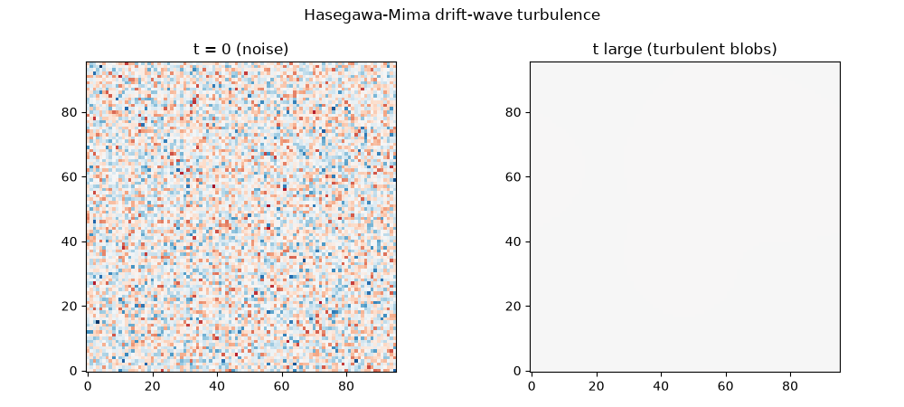
axes[0].imshow(phi0.T, origin="lower", cmap="RdBu_r", vmin=-vmax, vmax=vmax)
axes[0].set_title("t = 0 (noise)")
axes[1].imshow(phi.T, origin="lower", cmap="RdBu_r", vmin=-vmax, vmax=vmax)
axes[1].set_title("t large (turbulent blobs)")
fig.suptitle("Hasegawa-Mima drift-wave turbulence")
fig.tight_layout()

plt.show()

Animating the self-organization

anim = pk.plasma.animate_drift_wave_turbulence(phi0, dt=0.02, steps_per_frame=40, n_frames=40, length=length)

plt.show()