Debye and Hückel: screening and the Debye length

Debye and Hückel (1923), studying electrolytes, asked what the potential around one ion looks like when the other mobile charges are free to rearrange. Charges of the opposite sign gather around it, those of the same sign are pushed away, and the Boltzmann-distributed cloud cancels the ion’s field beyond a characteristic distance, the Debye length

\[\lambda_D = \sqrt{\frac{\varepsilon_0 k_BT}{n e^2}} = \frac{v_{th}}{\omega_p}.\]

Linearizing the Poisson-Boltzmann equation gives the screened, Yukawa potential \(\phi = \frac{q}{4\pi\varepsilon_0 r}e^{-r/\lambda_D}\). Plasma physics adopted the result unchanged. This example solves the full nonlinear Poisson-Boltzmann equation around a test charge, compares it with the Debye-Hückel form, and tabulates \(\lambda_D\) and the number of particles in a Debye sphere for real plasmas using plasma_frequency().

import matplotlib.pyplot as plt
import numpy as np
from scipy.integrate import solve_bvp

from physicskit.constants import ELECTRON_MASS, ELEMENTARY_CHARGE, K_B, VACUUM_PERMITTIVITY
from physicskit.plasma.waves import plasma_frequency

The screened potential

In units \(\psi = e\phi/k_BT\) and \(x = r/\lambda_D\), with Boltzmann electrons around a fixed positive test charge on a uniform ion background,

\[\psi'' + \frac{2}{x}\psi' = e^{\psi} - 1,\]

with the bare Coulomb field \(\psi' = -Q/x^2\) at the core and \(\psi\to0\) far away. \(Q\) measures the test charge’s strength against the thermal energy. For small \(Q\) the solution is Debye-Hückel’s \(\psi = Q e^{-x}/x\); for large \(Q\) the electrons pile up nonlinearly close in.

x_core, x_far = 0.05, 12.0
x = np.geomspace(x_core, x_far, 400)


def solve(Q):
    def rhs(xx, y):
        return np.vstack([y[1], np.expm1(y[0]) - 2 * y[1] / xx])

    def bc(ya, yb):
        return np.array([ya[1] + Q / x_core**2, yb[0]])

    guess = np.vstack([Q * np.exp(-x) / x, -Q * np.exp(-x) * (1 + x) / x**2])
    sol = solve_bvp(rhs, bc, x, guess, tol=1e-6, max_nodes=100000)
    return sol.sol(x)[0]


fig1, (ax1, ax2) = plt.subplots(1, 2, figsize=(11, 4))
for Q, color in [(0.01, "steelblue"), (0.5, "darkorange"), (3.0, "firebrick")]:
    psi = solve(Q)
    debye = Q * np.exp(-x) / x
    ax1.loglog(x, psi / Q, color=color, label=f"Poisson-Boltzmann, Q = {Q}")
    ax2.semilogx(x, psi / debye, color=color, label=f"Q = {Q}")
    i1 = np.argmin(np.abs(x - 1))
    print(f"Q = {Q:5}: psi / Debye-Huckel at r = lambda_D: {psi[i1] / debye[i1]:.3f}")
ax1.loglog(x, 1 / x, "k:", label="bare Coulomb 1/x")
ax1.loglog(x, np.exp(-x) / x, "k--", label=r"Debye-Hückel $e^{-x}/x$")
ax1.set_ylim(1e-6, 30)
ax1.set_xlabel(r"$r/\lambda_D$")
ax1.set_ylabel(r"$\psi / Q$")
ax1.set_title("A test charge, screened")
ax1.legend(fontsize=7)
ax2.axhline(1, color="k", lw=0.8)
ax2.set_xlabel(r"$r/\lambda_D$")
ax2.set_ylabel("Poisson-Boltzmann / Debye-Hückel")
ax2.set_title("Linear theory holds for weak charges")
ax2.legend(fontsize=8)
fig1.tight_layout()

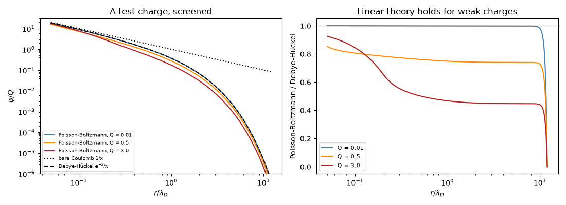
Q =  0.01: psi / Debye-Huckel at r = lambda_D: 0.999
Q =   0.5: psi / Debye-Huckel at r = lambda_D: 0.749
/Users/cpoli/Code/physicskit/examples/plasma/waves/plot_04_debye_screening.py:54: RuntimeWarning: overflow encountered in expm1
  return np.vstack([y[1], np.expm1(y[0]) - 2 * y[1] / xx])
/Users/cpoli/Code/physicskit/.venv/lib/python3.12/site-packages/scipy/integrate/_bvp.py:41: RuntimeWarning: invalid value encountered in subtract
  df_dy[:, i, :] = (f_new - f0) / hi
/Users/cpoli/Code/physicskit/.venv/lib/python3.12/site-packages/scipy/integrate/_bvp.py:567: RuntimeWarning: invalid value encountered in divide
  r_middle /= 1 + np.abs(f_middle)
/Users/cpoli/Code/physicskit/.venv/lib/python3.12/site-packages/scipy/integrate/_bvp.py:568: RuntimeWarning: invalid value encountered in divide
  r1 /= 1 + np.abs(f1)
/Users/cpoli/Code/physicskit/.venv/lib/python3.12/site-packages/scipy/integrate/_bvp.py:569: RuntimeWarning: invalid value encountered in divide
  r2 /= 1 + np.abs(f2)
Q =   3.0: psi / Debye-Huckel at r = lambda_D: 0.468

Debye lengths of real plasmas

\(\lambda_D = v_{th}/\omega_p\) with \(v_{th}=\sqrt{k_BT/m_e}\). A gas is a plasma only if \(\lambda_D\) is much smaller than the system and a Debye sphere holds many particles, \(N_D = \tfrac43\pi n\lambda_D^3 \gg 1\), so the screening cloud is a smooth crowd rather than a few individuals. The dense solar core is the marginal case: only a handful of electrons per Debye sphere.

plasmas = {
    "ionosphere": (1e11, 1e3),
    "solar corona": (1e15, 1e6),
    "tokamak core": (1e20, 1e8),
    "solar core": (1e32, 1.5e7),
    "interstellar medium": (1e6, 1e4),
}
print(f"\n{'plasma':20s} {'n [m^-3]':>9s} {'T [K]':>8s} {'lambda_D':>12s} {'N_D':>9s}")
lam, ND = {}, {}
for name, (n, T) in plasmas.items():
    v_th = np.sqrt(K_B * T / ELECTRON_MASS)
    lam[name] = v_th / plasma_frequency(n, ELEMENTARY_CHARGE, ELECTRON_MASS)
    ND[name] = 4 / 3 * np.pi * n * lam[name] ** 3
    print(f"{name:20s} {n:9.0e} {T:8.0e} {lam[name]:10.2e} m {ND[name]:9.1e}")

fig2, ax3 = plt.subplots(figsize=(6, 4))
for name in plasmas:
    ax3.loglog(lam[name], ND[name], "o", ms=8)
    ax3.annotate(name, (lam[name], ND[name]), textcoords="offset points", xytext=(6, 4), fontsize=8)
ax3.axhline(1, color="k", ls=":", label=r"$N_D = 1$")
ax3.set_xlabel(r"Debye length $\lambda_D$ [m]")
ax3.set_ylabel(r"particles per Debye sphere $N_D$")
ax3.set_title("Particles per Debye sphere")
ax3.legend(fontsize=8)
fig2.tight_layout()

plt.show()

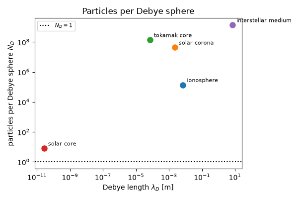
plasma                n [m^-3]    T [K]     lambda_D       N_D
ionosphere               1e+11    1e+03   6.90e-03 m   1.4e+05
solar corona             1e+15    1e+06   2.18e-03 m   4.4e+07
tokamak core             1e+20    1e+08   6.90e-05 m   1.4e+08
solar core               1e+32    2e+07   2.67e-11 m   8.0e+00
interstellar medium      1e+06    1e+04   6.90e+00 m   1.4e+09

Check

Weak charges are screened as Debye-Hückel’s e^(-r/lambda_D)/r; strong ones beyond it (nonlinear Poisson-Boltzmann). lambda_D = sqrt(eps0 k T / n e^2), N_D = (4/3) pi n lambda_D^3.

i1 = np.argmin(np.abs(x - 1))
ratios = {Q: solve(Q)[i1] / (Q * np.exp(-x[i1]) / x[i1]) for Q in (0.01, 3.0)}
assert abs(ratios[0.01] - 1) < 0.005 and ratios[3.0] < 0.6
for name, (n, T) in plasmas.items():
    assert abs(lam[name] / np.sqrt(VACUUM_PERMITTIVITY * K_B * T / (n * ELEMENTARY_CHARGE**2)) - 1) < 1e-10
    assert abs(ND[name] - 4 / 3 * np.pi * n * lam[name] ** 3) < 1e-9 * ND[name]