Hartree-Fock: the self-consistent field for H₂ and helium

Hartree (1928) let each electron move in the average field of all the others and iterated until the field reproduced itself. Fock and Slater (1930) added the exchange term required by the antisymmetry of the wavefunction. restricted_hartree_fock() solves the resulting Roothaan equations \(FC = SC\varepsilon\). This example follows the SCF iterations for helium, converges helium to the Hartree-Fock limit \(-2.86168\) hartree with growing Gaussian bases, and traces the \(\mathrm H_2\) bond, including the well-known failure of restricted Hartree-Fock at dissociation.

import matplotlib.pyplot as plt
import numpy as np

from physicskit.quantum.chapters.hartree_fock import (
    even_tempered_s_basis,
    kinetic_matrix,
    nuclear_attraction_matrix,
    restricted_hartree_fock,
    sto3g_1s,
)

origin = np.zeros(3)
E_HF_LIMIT = -2.8616800  # helium, Clementi and Roetti (1974)
E_EXACT_HE = -2.9037244  # nonrelativistic exact (Pekeris 1959)

Helium: approaching the Hartree-Fock limit

Every basis gives an energy above the Hartree-Fock limit (the variational principle), approaching it as even-tempered s functions are added. The remaining gap to the exact energy, about 0.042 hartree, is the correlation energy that Hartree-Fock misses by construction.

# each set uses ratio 2.5, centered within the exponent window of the 14-function set
sizes = np.arange(2, 15)
E_he = [restricted_hartree_fock(even_tempered_s_basis(origin, n, 0.05 * 2.5 ** ((14 - n) / 2), 2.5), [2], [origin], 2).energy for n in sizes]
E_sto3g = restricted_hartree_fock([sto3g_1s(1.69, origin)], [2], [origin], 2).energy

fig, axes = plt.subplots(1, 2, figsize=(12, 4.5))
axes[0].semilogy(sizes, np.array(E_he) - E_HF_LIMIT, "o-", label="even-tempered s basis")
axes[0].axhline(E_sto3g - E_HF_LIMIT, color="C1", ls="--", label=f"STO-3G ({E_sto3g:.4f})")
axes[0].axhline(E_HF_LIMIT - E_EXACT_HE, color="C3", ls=":", label="|correlation energy|")
axes[0].set_xlabel("number of basis functions")
axes[0].set_ylabel(r"$E - E_{\rm HF\ limit}$ (hartree)")
axes[0].set_title("Helium: variational convergence to the HF limit")
axes[0].legend(fontsize=8)
print(f"He, 14 s functions: E = {E_he[-1]:.6f} hartree (HF limit {E_HF_LIMIT})")

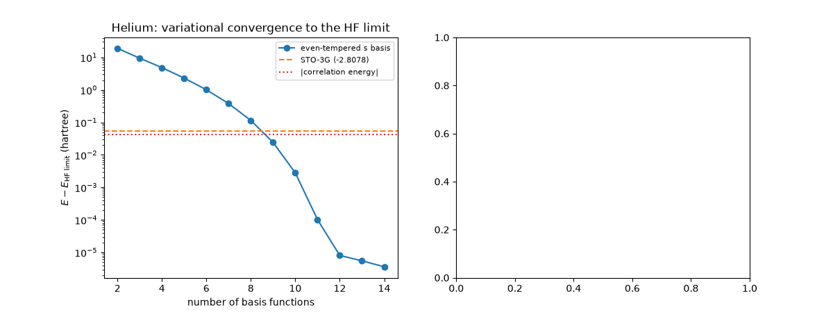
He, 14 s functions: E = -2.861676 hartree (HF limit -2.86168)

The self-consistent iterations

Starting from the core-Hamiltonian guess (no electron repulsion), each iteration rebuilds the Fock operator from the current orbitals.

basis = even_tempered_s_basis(origin, 10, 0.05, 2.5)
history = [restricted_hartree_fock(basis, [2], [origin], 2, max_iter=k, tol=0.0).energy for k in range(1, 13)]
axes[1].semilogy(range(1, 13), np.abs(np.array(history) - history[-1]) + 1e-16, "o-")
axes[1].set_xlabel("SCF iteration")
axes[1].set_ylabel(r"$|E_k - E_{\rm converged}|$")
axes[1].set_title("SCF convergence for helium")
fig.tight_layout()

The hydrogen molecule in STO-3G

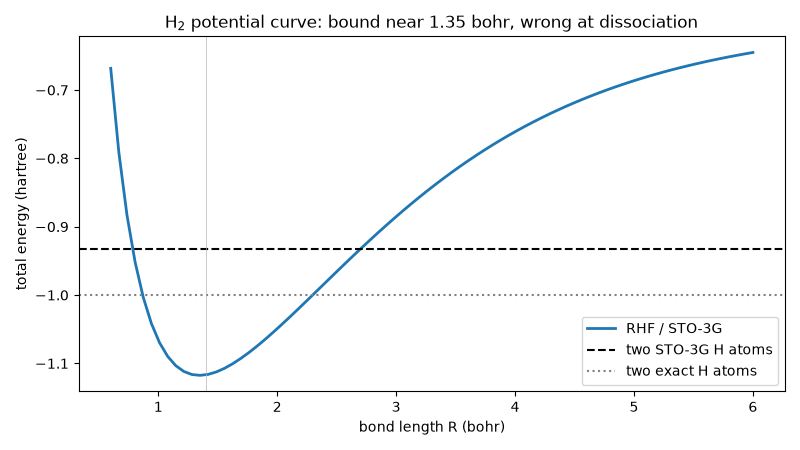
Near equilibrium the minimal basis reproduces Szabo and Ostlund’s \(E = -1.1167\) hartree at \(R = 1.4\) bohr. Pulled apart, the closed-shell determinant keeps both electrons in the same bonding orbital, which is half ionic (\(\mathrm{H^+H^-}\)), so the energy rises far above that of two separate hydrogen atoms. Fixing this needs a multi-determinant (correlated) wavefunction.

R = np.linspace(0.6, 6.0, 80)
E_h2 = []
for r in R:
    pos = np.array([[0.0, 0.0, 0.0], [r, 0.0, 0.0]])
    E_h2.append(restricted_hartree_fock([sto3g_1s(1.24, p) for p in pos], [1, 1], pos, 2).energy)
h = [sto3g_1s(1.24, origin)]
E_H = (kinetic_matrix(h) + nuclear_attraction_matrix(h, [1.0], [origin]))[0, 0]

fig2, ax2 = plt.subplots(figsize=(8, 4.5))
ax2.plot(R, E_h2, lw=2, label="RHF / STO-3G")
ax2.axhline(2 * E_H, color="k", ls="--", label="two STO-3G H atoms")
ax2.axhline(-1.0, color="0.5", ls=":", label="two exact H atoms")
ax2.axvline(1.4, color="0.7", lw=0.5)
ax2.set_xlabel("bond length R (bohr)")
ax2.set_ylabel("total energy (hartree)")
ax2.set_title(r"H$_2$ potential curve: bound near 1.35 bohr, wrong at dissociation")
ax2.legend()
fig2.tight_layout()

Check

The largest basis reaches the Clementi-Roetti Hartree-Fock limit; every basis stays variational (above it); the remaining gap to Pekeris’ exact energy is the correlation energy, -0.042 hartree. The STO-3G H2 minimum sits near the textbook R = 1.346 bohr, E = -1.117 hartree.

assert abs(E_he[-1] - E_HF_LIMIT) < 1e-4
assert np.all(np.array(E_he) > E_HF_LIMIT - 1e-6) and E_sto3g > E_HF_LIMIT
assert abs((E_HF_LIMIT - E_EXACT_HE) - 0.042) < 1e-3
assert abs(R[np.argmin(E_h2)] - 1.346) < 0.07
assert abs(min(E_h2) + 1.117) < 0.002