The harmonic oscillator suite#

Four canonical states of the 1D quantum harmonic oscillator

\[\hat H = \frac{\hat p^2}{2m} + \frac{1}{2} m \omega^2 \hat x^2, \qquad E_n = \hbar\omega\left(n+\tfrac12\right),\]

each highlighting a different piece of the oscillator’s physics. Fock (energy) eigenstates $\phi_n(x)$ are stationary: their probability density never changes shape, only the energy level $E_n$ differs. Glauber coherent states $\lvert\alpha\rangle$, the Poissonian superposition $\psi_\alpha(x,t)=\sum_n c_n\phi_n(x)e^{-iE_nt/\hbar}$ with $c_n = e^{-\lvert\alpha\rvert^2/2}\alpha^n/\sqrt{n!}$, instead keep a fixed Gaussian shape that oscillates rigidly back and forth, tracing the classical trajectory. Squeezed vacuum states redistribute the zero-point uncertainty between the quadratures while preserving the minimum-uncertainty product, $\Delta x^2 = (\hbar/2m\omega)\,e^{-2r}$ shrinking as $\Delta p^2 = (\hbar m\omega/2)\,e^{2r}$ grows with the squeezing parameter $r$. Finally, a thermal (mixed) state at temperature $T$ incoherently populates the Fock ladder according to the Boltzmann weights, broadening the position distribution $P(x)$ well beyond the $T=0$ ground-state width as $T$ increases.

import matplotlib.pyplot as plt
import numpy as np

from physicskit.quantum.chapters.harmonic_spin import HarmonicOscillator, ThermalState
from physicskit.quantum.visualizers.phase_space import WignerVisualizer
from physicskit.quantum.visualizers.wavefunctions import animate_density

ho = HarmonicOscillator()
x = np.linspace(-8, 8, 100)
V = 0.5 * ho.m * ho.omega**2 * x**2

Fock states with the potential and energy levels, a coherent state’s rigid oscillation, squeezed-vacuum quadrature squeezing, and thermal broadening. ————————————————————————– Top-left: the potential $V(x)$ with the first four Fock eigenfunctions $\phi_n(x)$ offset to their energies $E_n$. Top-right: a coherent state’s probability density at several times over one period, translating without changing shape. Bottom-left: the squeezed-vacuum density for increasing $r$, narrowing in $x$ at the cost of momentum spread. Bottom-right: the thermal position distribution $P(x)$ for increasing temperature $T$.

fig, axes = plt.subplots(2, 2, figsize=(11, 9))

# Fock states |n>, shown with the potential V(x) and their energy levels E_n
axes[0, 0].plot(x, V, color="black", lw=1, label="V(x)")
for n in range(4):
    axes[0, 0].axhline(ho.energy(n), color="gray", lw=0.5, ls=":")
    axes[0, 0].plot(x, ho.energy(n) + ho.eigenfunction(n, x), label=f"n={n}")
axes[0, 0].set_ylim(-0.5, 5)
axes[0, 0].set_title(r"Fock states $|n\rangle$ (with $V(x)=\frac{1}{2}m\omega^2x^2$ and $E_n$)")
axes[0, 0].legend(fontsize=8)

# Coherent state |alpha>: fixed shape, oscillating center
alpha = 3.0
times = np.linspace(0, 2 * np.pi / ho.omega, 6)
for t in times:
    psi_t = ho.coherent_wavefunction(alpha, x, t=t)
    axes[0, 1].plot(x, np.abs(psi_t) ** 2 + 0.15 * t, label=f"t={t:.2f}")
axes[0, 1].set_title(r"Coherent state $|\alpha\rangle$: fixed shape, oscillating center")
axes[0, 1].legend(fontsize=6, ncol=2)

# Squeezed vacuum: quadrature squeezing
for r in [0.0, 0.5, 1.0]:
    psi_sq = ho.squeezed_vacuum_wavefunction(x, r)
    axes[1, 0].plot(x, np.abs(psi_sq) ** 2, label=f"r={r}")
    dx, dp = ho.squeezed_uncertainties(r)
    print(f"r={r}: dx={dx:.4f}, dp={dp:.4f}, dx*dp={dx * dp:.6f} (hbar/2={ho.hbar / 2})")
axes[1, 0].set_title(r"Squeezed vacuum: $\Delta x$ shrinks, $\Delta p$ grows")
axes[1, 0].legend(fontsize=8)

# Thermal broadening
for T in [0.1, 1.0, 3.0]:
    thermal = ThermalState(ho, T=T)
    axes[1, 1].plot(x, thermal.position_distribution(x), label=f"T={T}")
axes[1, 1].set_title(r"Thermal state: $P(x)$ broadens with $T$")
axes[1, 1].legend(fontsize=8)

for ax in axes.flat:
    ax.set_xlabel("x")

fig.tight_layout()

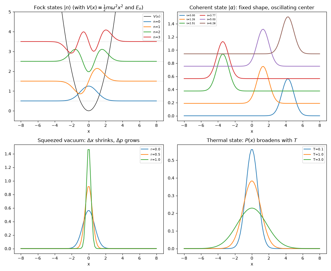
$Fock states $|n\rangle$ (with $V(x)=\frac{1}{2}m\omega^2x^2$ and $E_n$), Coherent state $|\alpha\rangle$: fixed shape, oscillating center, Squeezed vacuum: $\Delta x$ shrinks, $\Delta p$ grows, Thermal state: $P(x)$ broadens with $T$$

r=0.0: dx=0.7071, dp=0.7071, dx*dp=0.500000 (hbar/2=0.5)
r=0.5: dx=0.4289, dp=1.1658, dx*dp=0.500000 (hbar/2=0.5)
r=1.0: dx=0.2601, dp=1.9221, dx*dp=0.500000 (hbar/2=0.5)

An animated Fock-state superposition#

Unlike a single stationary Fock state (whose density is time-independent) or a coherent state (a rigidly oscillating Gaussian), a generic superposition of Fock eigenstates genuinely reshapes over time, beating at every pairwise frequency $(E_{n_k}-E_{n_j})/\hbar$. superposition_trajectory() builds this time-evolved superposition, and animate_density() renders it frame by frame, phase-colored.

t_anim = np.linspace(0, 2 * np.pi / ho.omega, 60)
frames = ho.superposition_trajectory([0, 1, 2], [1.0, 1.0j, 0.5], x, t_anim)
anim = animate_density(x, frames, times=t_anim)
# anim.save("harmonic_superposition.gif", writer="pillow", fps=15)

Coherent vs. squeezed states in phase space: a circular blob vs. an ellipse#

The coherent- and squeezed-state densities above are both position-space projections of the same states; WignerVisualizer shows them in phase space directly instead. A coherent state’s Wigner function is a circular Gaussian blob, displaced from the origin but otherwise identical in shape to the vacuum – minimum uncertainty, isotropic in $x$ and $p$. The squeezed vacuum’s is an ellipse: squeezed in $x$ and stretched in $p$ by the same $e^{\mp2r}$ factors plotted above, with its total area preserved.

wv = WignerVisualizer(n_p=160)
x_ph = np.linspace(-6, 14, 240)


def _denoise(W):
    # coherent_wavefunction sums a truncated Fock series; the residual
    # truncation error is negligible in amplitude (~1e-7 of the peak) but
    # still oscillates in sign, which a fixed-level contourf would
    # otherwise render as spurious fringes far from the actual blob.
    return np.where(np.abs(W) < 1e-6 * np.abs(W).max(), 0.0, W)


fig4, axes4 = plt.subplots(1, 2, figsize=(11, 4.5))

psi_coh = ho.coherent_wavefunction(alpha, x_ph, t=0.0)
xg_c, pg_c, W_coh = wv.compute(x_ph, psi_coh, p_max=8.0)
wv.plot_contour(xg_c, pg_c, _denoise(W_coh), ax=axes4[0])
axes4[0].set_title(f"Coherent state $|\\alpha={alpha}\\rangle$\n(circular blob, displaced from the origin)")

r_wigner = 1.0
psi_sq = ho.squeezed_vacuum_wavefunction(x_ph, r_wigner)
xg_s, pg_s, W_sq = wv.compute(x_ph, psi_sq, p_max=8.0)
wv.plot_contour(xg_s, pg_s, W_sq, ax=axes4[1])
axes4[1].set_title(f"Squeezed vacuum (r={r_wigner})\n(ellipse: squeezed in x, stretched in p)")

fig4.tight_layout()

print(f"min W of the coherent-state Wigner function (should stay >=0): {W_coh.min():.2e}")
print(f"min W of the squeezed-vacuum Wigner function (should stay >=0): {W_sq.min():.2e}")

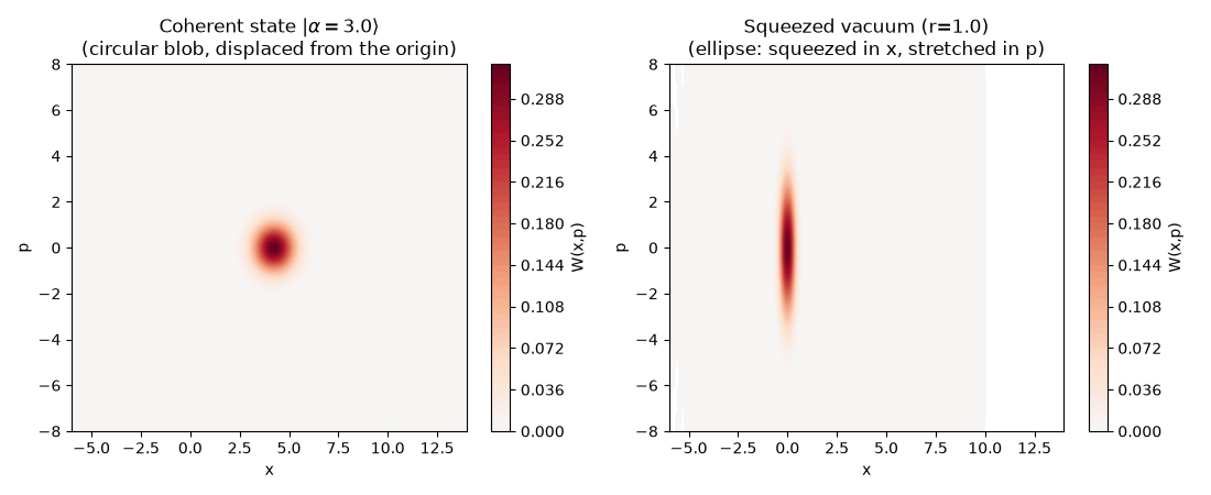
$Coherent state $|\alpha=3.0\rangle$ (circular blob, displaced from the origin), Squeezed vacuum (r=1.0) (ellipse: squeezed in x, stretched in p)$

min W of the coherent-state Wigner function (should stay >=0): -7.08e-14
min W of the squeezed-vacuum Wigner function (should stay >=0): -1.40e-92

Total running time of the script: (0 minutes 7.689 seconds)

Gallery generated by Sphinx-Gallery