Hydrogen orbitals

The hydrogen-atom eigenstates factor into a radial part and a spherical harmonic,

\[\psi_{nlm}(r,\theta,\phi) = R_{nl}(r)\, Y_l^m(\theta,\phi), \qquad E_n = -\frac{Z^2}{2n^2}\ \text{(Hartree)},\]

labeled by the principal, orbital, and magnetic quantum numbers \(n, l, m\) (with \(0\le l<n\) and \(\lvert m\rvert\le l\)); \(E_n\) depends on \(n\) alone, so states sharing \(n\) but differing in \(l,m\) are degenerate. This example plots the radial probability density \(r^2\lvert R_{nl}(r)\rvert^2\) for a few \((n,l,m)\) combinations, the resulting energy ladder converging to the ionization threshold \(E\to0\) as \(n\to\infty\), a volumetric \(\lvert\psi_{2,1,0}\rvert^2\) electron-density cloud, and a coherent superposition of two different eigenstates whose density beats in time rather than staying static.

import matplotlib.pyplot as plt
import numpy as np

from physicskit.quantum.chapters.hydrogen_am import HydrogenOrbital
from physicskit.quantum.visualizers.orbitals import animate_orbital_beating, plot_orbital_cloud

Radial densities and the energy-level ladder

fig, (ax, ax_levels) = plt.subplots(1, 2, figsize=(12, 5), gridspec_kw={"width_ratios": [2, 1]})
r = np.linspace(1e-6, 30, 2000)

for n, l, m in [(1, 0, 0), (2, 0, 0), (2, 1, 0), (3, 2, 1)]:
    orb = HydrogenOrbital(n, l, m)
    ax.plot(r, orb.radial_density(r), label=f"n={n}, l={l}, m={m}  (E={orb.energy:.4f})")
    print(f"n={n} l={l} m={m}: normalization={orb.check_normalization():.6f}, most probable r={orb.most_probable_radius():.3f}")

ax.set_xlabel("r (Bohr radii)")
ax.set_ylabel(r"$r^2 |R_{nl}(r)|^2$")
ax.set_title("Hydrogen radial probability densities")
ax.legend(fontsize=8)

# Energy-level ladder E_n = -1/(2n^2), converging to the n->infinity ionization limit
for n in range(1, 6):
    E_n = HydrogenOrbital(n, 0, 0).energy
    ax_levels.axhline(E_n, xmin=0.1, xmax=0.9, color="C0", lw=2)
    ax_levels.text(0.92, E_n, f"n={n}", va="center", fontsize=8)
ax_levels.axhline(0.0, color="gray", ls="--", lw=0.8)
ax_levels.text(0.92, 0.0, "ionized", va="center", fontsize=8, color="gray")
ax_levels.set_xlim(0, 1.3)
ax_levels.set_xticks([])
ax_levels.set_ylabel(r"$E_n = -Z^2/(2n^2)$  (Hartree)")
ax_levels.set_title("Energy-level ladder")

fig.tight_layout()

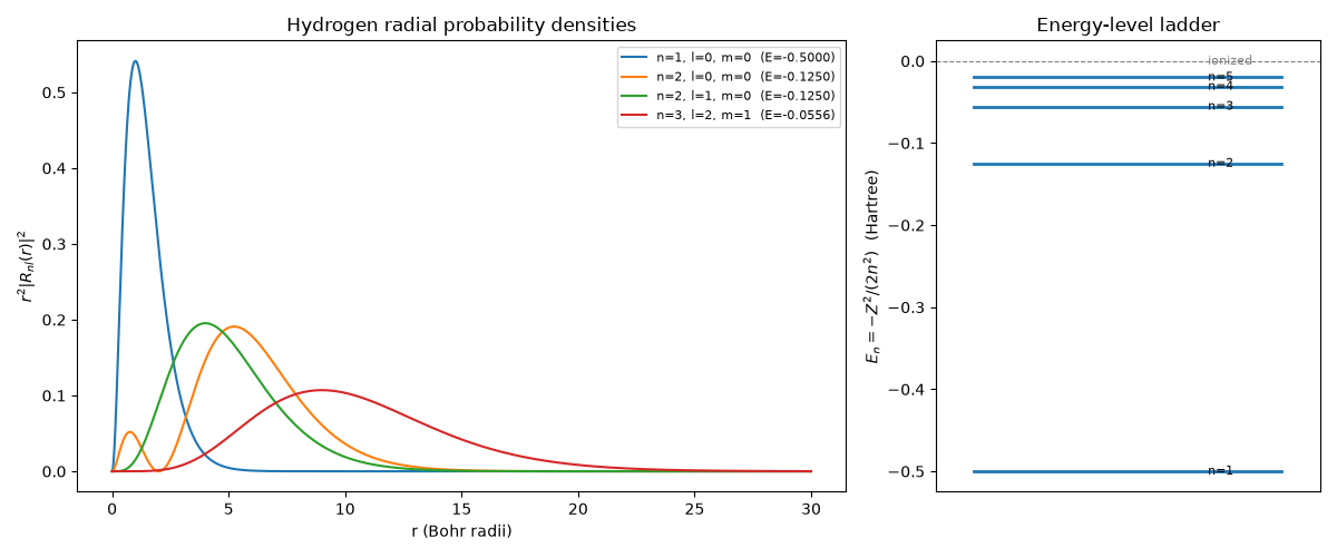
n=1 l=0 m=0: normalization=1.000000, most probable r=1.000
n=2 l=0 m=0: normalization=1.000000, most probable r=5.237
n=2 l=1 m=0: normalization=1.000000, most probable r=4.000
n=3 l=2 m=1: normalization=1.000000, most probable r=9.000

A volumetric \(\lvert\psi_{2,1,0}\rvert^2\) electron-density cloud

plot_orbital_cloud() returns an interactive Plotly figure; call .show() or .write_html(...) on it to view or export it.

orb_2p = HydrogenOrbital(2, 1, 0)
fig3d = plot_orbital_cloud(orb_2p, n_points=45)

A coherent superposition of two eigenstates, beating in time

A single orbital’s density is static (an eigenstate of a time-independent Hamiltonian), but a coherent superposition of two eigenstates is not: orbital_superposition_density() genuinely reshapes at the Bohr frequency \(\omega_{ab}=E_a-E_b\). animate_orbital_beating() renders this as a Plotly frames-based isosurface animation with a Play button, stepping through one full beat period.

orb_a = HydrogenOrbital(2, 0, 0)
orb_b = HydrogenOrbital(3, 1, 0)
beat_period = 2 * np.pi / abs(orb_b.energy - orb_a.energy)
times_beat = np.linspace(0, beat_period, 24)

fig_beat = animate_orbital_beating(orb_a, orb_b, times_beat, n_points=35)