Wilson-Sommerfeld quantization: elliptical orbits and fine structure

Bohr quantized only circular orbits. Wilson (1915) and Sommerfeld (1916) generalized his rule to any periodic motion: every separable degree of freedom’s action around one cycle is a whole number of Planck constants,

\[\oint p_r\,dr = n_r h, \qquad \oint p_\varphi\,d\varphi = k h .\]

For the hydrogen atom this admits elliptical orbits labelled by \((n_r, k)\). Their energy depends only on \(n = n_r + k\), so Bohr’s levels come out unchanged but now contain several orbit shapes each. Sommerfeld then quantized the relativistic Kepler problem and found that the ellipses of one \(n\) split slightly in energy, which explained hydrogen’s fine structure. This example evaluates the radial action numerically with turning_points() and wkb_action(), draws the quantized ellipses, and compares Sommerfeld’s fine-structure formula with Dirac’s.

import matplotlib.pyplot as plt
import numpy as np
from scipy.optimize import brentq

from physicskit.semiclassical.core.wkb import turning_points, wkb_action

# Atomic units: hbar = m_e = e^2/(4 pi eps0) = 1, so h = 2 pi and E is in hartrees.
HARTREE_EV = 27.211386
ALPHA = 1 / 137.035999

Quantizing the radial motion

With angular momentum \(L = k\hbar\) fixed by the second condition, the radial motion lives in \(V_{\rm eff}(r) = -1/r + k^2/2r^2\). Solve \(\oint p_r\,dr = 2\int_{r_1}^{r_2}p_r\,dr = n_r h\) for the energy.

def radial_action(E, k):
    V = lambda r: -1.0 / r + k**2 / (2 * r**2)  # noqa: E731
    r1, r2 = turning_points(E, V, 1e-3, 400.0, n_search=20000)[:2]
    return 2 * wkb_action(E, V, 1.0, r1, r2)


print(f"{'n_r':>3s} {'k':>2s} {'n':>2s} {'E (numerical) [eV]':>19s} {'-13.606/n^2 [eV]':>17s}")
for n_total in (1, 2, 3):
    for k in range(1, n_total + 1):
        n_r = n_total - k
        E_circle = -1 / (2 * k**2)  # bottom of V_eff: the circular orbit, n_r = 0
        E = brentq(lambda E: radial_action(E, k) - 2 * np.pi * n_r, E_circle * (1 - 1e-2), -0.01) if n_r > 0 else E_circle
        print(f"{n_r:3d} {k:2d} {n_total:2d} {E * HARTREE_EV:19.4f} {-HARTREE_EV / 2 / n_total**2:17.4f}")

n_r  k  n  E (numerical) [eV]  -13.606/n^2 [eV]
  0  1  1            -13.6057          -13.6057
  1  1  2             -3.4014           -3.4014
  0  2  2             -3.4014           -3.4014
  2  1  3             -1.5117           -1.5117
  1  2  3             -1.5117           -1.5117
  0  3  3             -1.5117           -1.5117

The quantized ellipses

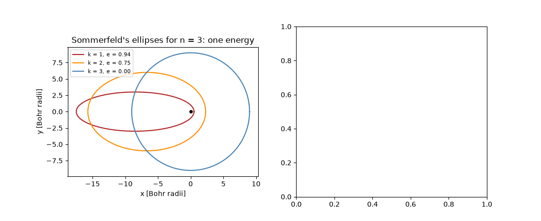
For principal number \(n\), the semi-major axis is \(a = n^2\) Bohr radii for every \(k\), and the semi-minor axis is \(b = nk\). \(k = n\) is Bohr’s circle; smaller \(k\) means a more eccentric orbit that dives closer to the nucleus. (\(k=0\) would pass straight through the nucleus and was excluded.)

fig, (ax1, ax2) = plt.subplots(1, 2, figsize=(11, 4.5))
phi = np.linspace(0, 2 * np.pi, 400)
n_total = 3
for k, color in zip(range(1, n_total + 1), ["firebrick", "darkorange", "steelblue"]):
    a, b = n_total**2, n_total * k
    e = np.sqrt(1 - (b / a) ** 2)
    r = a * (1 - e**2) / (1 + e * np.cos(phi))
    ax1.plot(r * np.cos(phi), r * np.sin(phi), color=color, label=f"k = {k}, e = {e:.2f}")
ax1.plot(0, 0, "ko", ms=4)
ax1.set_aspect("equal")
ax1.set_xlabel("x [Bohr radii]")
ax1.set_ylabel("y [Bohr radii]")
ax1.set_title(f"Sommerfeld's ellipses for n = {n_total}: one energy")
ax1.legend(fontsize=8)

<matplotlib.legend.Legend object at 0x17543d700>

Sommerfeld’s fine structure

Relativistically the ellipse precesses and the degeneracy breaks:

\[E_{n_r,k} = mc^2\left[1 + \frac{\alpha^2}{\left(n_r + \sqrt{k^2-\alpha^2}\right)^2}\right]^{-1/2} - mc^2 .\]

Dirac’s 1928 equation gives the same formula with \(k\) replaced by \(j+\tfrac12\), so Sommerfeld’s old-quantum-theory answer matches the exact one level by level, a famous coincidence.

MC2_EV = 510998.95


def sommerfeld(n_r, k):
    return MC2_EV * (1 / np.sqrt(1 + ALPHA**2 / (n_r + np.sqrt(k**2 - ALPHA**2)) ** 2) - 1)


def dirac(n, j):
    kappa = j + 0.5
    return MC2_EV * (1 / np.sqrt(1 + ALPHA**2 / (n - kappa + np.sqrt(kappa**2 - ALPHA**2)) ** 2) - 1)


print("\nfine-structure splittings (Sommerfeld vs Dirac):")
for n_total in (2, 3):
    E_k = [sommerfeld(n_total - k, k) for k in range(1, n_total + 1)]
    E_j = [dirac(n_total, k - 0.5) for k in range(1, n_total + 1)]
    for k in range(1, n_total + 1):
        shift = (E_k[k - 1] - (-13.605693 / n_total**2)) * 1e6
        print(f"  n={n_total}, k={k} (j={k - 0.5}): {shift:8.2f} micro-eV from Bohr; |Sommerfeld - Dirac| = {abs(E_k[k - 1] - E_j[k - 1]):.1e} eV")
    split = (E_k[1] - E_k[0]) / 4.135667696e-15 / 1e9
    print(f"  n={n_total}: k=1 to k=2 splitting {split:.2f} GHz")
    ax2.plot(range(1, n_total + 1), [(E - E_k[0]) * 1e6 for E in E_k], "o-", label=f"n = {n_total}")
ax2.set_xlabel("azimuthal quantum number k")
ax2.set_ylabel(r"energy above the k = 1 level [$\mu$eV]")
ax2.set_title("Relativistic splitting of each Bohr level")
ax2.set_xticks([1, 2, 3])
ax2.legend(fontsize=8)
fig.tight_layout()

plt.show()

fine-structure splittings (Sommerfeld vs Dirac):
  n=2, k=1 (j=0.5):   -56.64 micro-eV from Bohr; |Sommerfeld - Dirac| = 0.0e+00 eV
  n=2, k=2 (j=1.5):   -11.36 micro-eV from Bohr; |Sommerfeld - Dirac| = 0.0e+00 eV
  n=2: k=1 to k=2 splitting 10.95 GHz
  n=3, k=1 (j=0.5):   -20.14 micro-eV from Bohr; |Sommerfeld - Dirac| = 0.0e+00 eV
  n=3, k=2 (j=1.5):    -6.72 micro-eV from Bohr; |Sommerfeld - Dirac| = 0.0e+00 eV
  n=3, k=3 (j=2.5):    -2.25 micro-eV from Bohr; |Sommerfeld - Dirac| = 0.0e+00 eV
  n=3: k=1 to k=2 splitting 3.24 GHz

Check

The quantized radial action gives Bohr’s -1/(2 n^2) for every elliptical orbit; Sommerfeld’s relativistic formula is exactly Dirac’s with k = j + 1/2; the n = 2 fine-structure splitting is 10.95 GHz.

for n_total, k in [(2, 1), (3, 1), (3, 2)]:
    E = brentq(lambda E: radial_action(E, k) - 2 * np.pi * (n_total - k), -1 / (2 * k**2) * (1 - 1e-2), -0.01)
    assert abs(E + 1 / (2 * n_total**2)) < 1e-4
for n_total in (2, 3):
    for k in range(1, n_total + 1):
        assert abs(sommerfeld(n_total - k, k) - dirac(n_total, k - 0.5)) < 1e-12
split_n2 = (sommerfeld(0, 2) - sommerfeld(1, 1)) / 4.135667696e-15 / 1e9
assert abs(split_n2 - 10.95) < 0.01