Floquet-driven box: time-dependent perturbation theory

Dirac’s time-dependent perturbation theory describes how a weak, time-dependent perturbation drives transitions between the unperturbed stationary states of a system; Fermi later gave the leading-order transition-rate result its “golden rule” name. The same machinery describes a system driven periodically in time, where transitions become resonant multiphoton processes whenever an integer number of drive quanta \(\hbar\omega\) bridges an energy gap.

An infinite square well \([0,L]\) driven by an oscillating dipole field,

\[V(x,t) = V_0\left(x - \frac{L}{2}\right)\cos(\omega t),\]

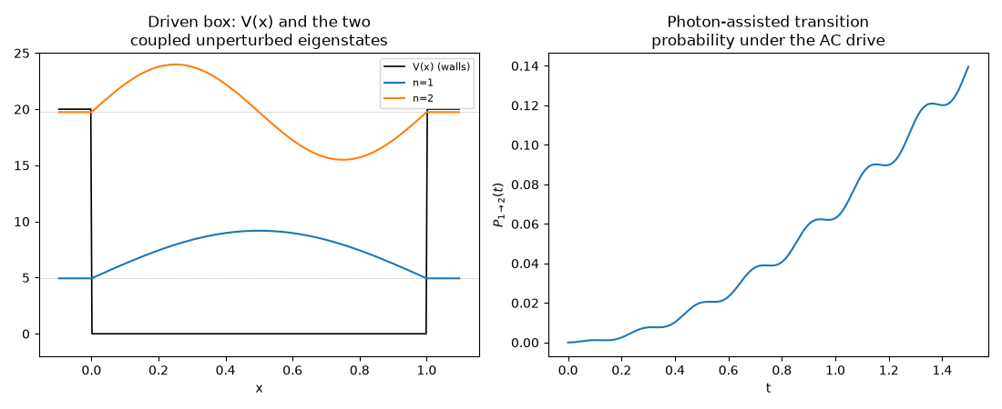
is propagated with the split-operator method starting from an unperturbed box eigenstate. When \(\hbar\omega\) (or a multiple of it) bridges the gap between two box levels, the drive induces resonant multiphoton (Rabi-like) transitions between them.

import matplotlib.pyplot as plt
import numpy as np

from physicskit.quantum.chapters.perturbation import FloquetDrivenBox

The driven box and a Floquet multiphoton transition

Left: the driven box’s confining potential \(V(x)\) together with its two lowest unperturbed eigenstates \(\psi_1,\psi_2\) (offset to their energies \(E_n = n^2\pi^2\hbar^2/(2mL^2)\)). Right: the resulting transition probability \(P_{1\to2}(t)\) as the driven box evolves from \(\psi_1\), oscillating at the multiphoton Rabi frequency set by the drive’s detuning from the \(1\to2\) gap.

fig, axes = plt.subplots(1, 2, figsize=(11, 4.5))

# Floquet-driven box: the well and its two coupled eigenstates
fb = FloquetDrivenBox(L=1.0, V0=3.0, omega=15.0, n_grid=512)
inside = (fb.x >= -0.1) & (fb.x <= 1.1)
wall = np.where((fb.x >= 0) & (fb.x <= fb.L), 0.0, 20.0)  # capped for display
axes[0].plot(fb.x[inside], wall[inside], color="black", lw=1.2, label="V(x) (walls)")
for n in (1, 2):
    axes[0].axhline(fb.box_energy(n), color="gray", lw=0.5, ls=":")
    axes[0].plot(fb.x[inside], fb.box_energy(n) + 3 * fb.box_eigenstate(n)[inside], label=f"n={n}")
axes[0].set_ylim(-2, 25)
axes[0].set_xlabel("x")
axes[0].set_title("Driven box: V(x) and the two\ncoupled unperturbed eigenstates")
axes[0].legend(fontsize=8)

# Floquet-driven box: multiphoton transition probability
times, probs = fb.transition_probability(1, 2, t_max=1.5, dt=2e-4)
axes[1].plot(times, probs)
axes[1].set_xlabel("t")
axes[1].set_ylabel(r"$P_{1 \to 2}(t)$")
axes[1].set_title("Photon-assisted transition\nprobability under the AC drive")

fig.tight_layout()

The Floquet chevron: transition probability vs. drive frequency and time

The single \(P_{1\to2}(t)\) curve above used one fixed drive frequency (\(\omega=15\), close to the unperturbed \(1\to2\) box gap); re-instantiating FloquetDrivenBox at each \(\omega\) on a grid around that gap and calling transition_probability() again traces out a Rabi-chevron-like resonance ridge in the \((\omega,t)\) plane, peaking sharply where the drive matches the gap.

omega_gap = fb.box_energy(2) - fb.box_energy(1)
omega_values = np.linspace(0.6 * omega_gap, 1.4 * omega_gap, 16)
t_grid = np.linspace(0, 3.0, 150)
P_chevron = np.zeros((len(omega_values), len(t_grid)))
for i, om in enumerate(omega_values):
    fb_om = FloquetDrivenBox(L=1.0, V0=3.0, omega=om, n_grid=256)
    times_om, probs_om = fb_om.transition_probability(1, 2, t_max=3.0, dt=5e-4)
    P_chevron[i] = np.interp(t_grid, times_om, probs_om)

fig2, ax3 = plt.subplots(figsize=(7, 4.5))
im = ax3.pcolormesh(t_grid, omega_values, P_chevron, shading="auto", cmap="inferno", vmin=0, vmax=1)
ax3.axhline(omega_gap, color="cyan", ls="--", lw=1, label=f"unperturbed 1->2 gap ({omega_gap:.2f})")
ax3.set_xlabel("t")
ax3.set_ylabel(r"drive frequency $\omega$")
ax3.set_title(r"Floquet chevron: $P_{1 \to 2}(t,\omega)$")
ax3.legend(fontsize=8)
fig2.colorbar(im, ax=ax3, label=r"$P_{1 \to 2}$")
fig2.tight_layout()

print(f"unperturbed 1->2 box gap: {omega_gap:.4f}")
print(f"peak P_1->2 in the chevron: {P_chevron.max():.4f} at omega={omega_values[np.argmax(P_chevron.max(axis=1))]:.4f}")

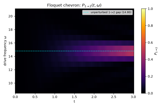
unperturbed 1->2 box gap: 14.8044
peak P_1->2 in the chevron: 0.4714 at omega=14.4096