2D quantum boxes

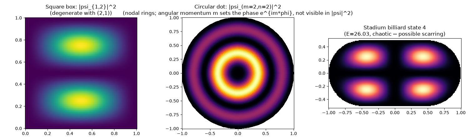
Three infinite-wall (“hard box”) potentials in two dimensions, each solved for its stationary states \(\psi(x,y)\) with \(\psi=0\) on the boundary. For the rectangular box \([0,L_x]\times[0,L_y]\), separation of variables gives closed-form modes with energies

\[E_{n_x,n_y} = \frac{\pi^2\hbar^2}{2m} \left(\frac{n_x^2}{L_x^2} + \frac{n_y^2}{L_y^2}\right);\]

when \(L_x=L_y\) (a square), distinct pairs \((n_x,n_y)\) and \((n_y,n_x)\) are degenerate. For a circular dot of radius \(R\), separation in polar coordinates instead gives Bessel-function eigenstates

\[\psi_{mn}(r,\phi) \propto J_{\lvert m\rvert}(k_{mn} r)\, e^{im\phi}, \qquad E_{mn} = \frac{\hbar^2 k_{mn}^2}{2m},\]

where \(k_{mn}R\) is the \(n\)-th positive zero of the order-\(\lvert m\rvert\) Bessel function \(J_{\lvert m\rvert}\) (so \(n\) counts radial nodal rings and \(m\) is the angular momentum quantum number). Finally, the Bunimovich stadium – a rectangle capped by two semicircles, whose classical billiard dynamics is chaotic – has no closed-form solution; its eigenstates are obtained by direct diagonalization of the finite-difference Laplacian on a grid, and can show scars: probability density that concentrates along unstable classical periodic orbits.

import matplotlib.pyplot as plt
import numpy as np

from physicskit.quantum.chapters.potentials import CircularBox2D, RectangularBox2D, StadiumBilliard2D

A square box mode, a circular dot’s Bessel mode, and a stadium billiard eigenstate. ————————————————————————– Left: probability density \(\lvert\psi_{n_x,n_y}\rvert^2\) for one square-box mode, degenerate with its \((n_y,n_x)\) partner. Middle: probability density \(\lvert\psi_{mn}\rvert^2\) for a circular-dot mode, showing \(n\) nodal rings (the angular phase \(e^{im\phi}\) does not appear in \(\lvert\psi\rvert^2\)). Right: a higher stadium eigenstate colored by \(\lvert\psi\rvert^2\), in the chaotic-billiard regime where scarring can occur.

fig, axes = plt.subplots(1, 3, figsize=(15, 4.5))

# Rectangular box: degeneracy for a square (Lx=Ly)
box = RectangularBox2D(Lx=1.0, Ly=1.0)
degeneracies = box.degeneracies(n_max=5)
print(f"Square box: {len(degeneracies)} degenerate energy levels among the first states, e.g.:")
for E, pairs in list(degeneracies.items())[:3]:
    print(f"  E={E:.4f}: (nx,ny) in {pairs}")

X, Y = box.grid(150)
state = box.spectrum(5)[1]
density = state.psi(X, Y, box.Lx, box.Ly) ** 2
axes[0].pcolormesh(X, Y, density, shading="auto", cmap="viridis")
axes[0].set_title(f"Square box: |psi_{{{state.nx},{state.ny}}}|^2\n(degenerate with ({state.ny},{state.nx}))")
axes[0].set_aspect("equal")

# Circular quantum dot: Bessel eigenstates
cb = CircularBox2D(R=1.0)
state = cb.eigenstate(m=2, n=2)
r, phi = cb.polar_grid(120, 150)
psi = state.psi(r, phi, cb.R)
Xc, Yc = r * np.cos(phi), r * np.sin(phi)
axes[1].pcolormesh(Xc, Yc, np.abs(psi) ** 2, shading="auto", cmap="inferno")
axes[1].set_title(f"Circular dot: |psi_(m={state.m},n={state.n})|^2\n(nodal rings; angular momentum m sets the phase e^{{im*phi}}, not visible in |psi|^2)")
axes[1].set_aspect("equal")

# Stadium billiard: quantum scars
sb = StadiumBilliard2D(L=1.0, R=0.5)
energies, wavefunctions, Xs, Ys, mask = sb.solve(n_points=220, n_states=6)
scar_idx = 4
density_s = wavefunctions[scar_idx] ** 2
density_s = np.where(mask, density_s, np.nan)
axes[2].pcolormesh(Xs, Ys, density_s, shading="auto", cmap="magma")
axes[2].set_title(f"Stadium billiard state {scar_idx}\n(E={energies[scar_idx]:.2f}, chaotic -- possible scarring)")
axes[2].set_aspect("equal")

fig.tight_layout()

Square box: 10 degenerate energy levels among the first states, e.g.:
  E=24.6740: (nx,ny) in [(1, 2), (2, 1)]
  E=49.3480: (nx,ny) in [(1, 3), (3, 1)]
  E=64.1524: (nx,ny) in [(2, 3), (3, 2)]
/Users/cpoli/Code/physicskit/examples/quantum/potentials/plot_2d_quantum_boxes.py:74: UserWarning: The input coordinates to pcolormesh are interpreted as cell centers, but are not monotonically increasing or decreasing. This may lead to incorrectly calculated cell edges, in which case, please supply explicit cell edges to pcolormesh.
  axes[1].pcolormesh(Xc, Yc, np.abs(psi) ** 2, shading="auto", cmap="inferno")