The expanding universe: Hubble’s law and the Friedmann equations

In 1929, Edwin Hubble found that distant galaxies recede from us at a rate proportional to their distance – direct observational evidence that the universe is expanding, exactly as Einstein’s field equations (applied to a homogeneous, isotropic universe by Friedmann and Lemaitre) had already predicted. Plugging the Friedmann-Lemaitre-Robertson-Walker metric into Einstein’s equations for a universe filled with radiation, matter, spatial curvature, and a cosmological constant \(\Lambda\) gives the Friedmann equation for the expansion rate \(H(a) = \dot a / a\) in terms of the scale factor \(a\) (normalized to \(a=1\) today):

\[\left(\frac{H(a)}{H_0}\right)^2 = \Omega_r a^{-4} + \Omega_m a^{-3} + \Omega_k a^{-2} + \Omega_\Lambda\]

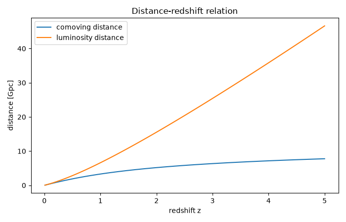
This example solves that equation for a near-flat \(\Lambda\text{CDM}\) universe with \(H_0 = 70\) km/s/Mpc, \(\Omega_m = 0.3\), \(\Omega_r = 9\times 10^{-5}\), and \(\Omega_\Lambda = 0.7\) (with the curvature term \(\Omega_k = 1 - \Omega_m - \Omega_r - \Omega_\Lambda\) fixed so the density parameters sum to the critical density today), showing how the scale factor \(a(t)\) has grown over cosmic history, and how the comoving distance \(D_C(z) = c \int_0^z dz' / H(z')\) and luminosity distance \(D_L = (1+z) D_C\) to a galaxy grow with its redshift \(z\).

import matplotlib.pyplot as plt
import numpy as np

from physicskit.relativity.chapters.cosmology import FLRWCosmology

The expansion history: scale factor versus cosmic time

cosmo = FLRWCosmology(H0=70.0, Omega_m=0.3, Omega_r=9.0e-5, Omega_Lambda=0.7)
t_gyr, a = cosmo.scale_factor_history(n_points=300, a_min=1.0e-3, a_max=3.0)
age_today = cosmo.age_gyr(1.0)

plt.figure(figsize=(7, 4.5))
plt.plot(t_gyr, a)
plt.axhline(1.0, color="k", linestyle="--", linewidth=1, alpha=0.5)
plt.axvline(
    age_today,
    color="crimson",
    linestyle="--",
    linewidth=1,
    alpha=0.7,
    label=f"today, t={age_today:.2f} Gyr",
)
plt.xlabel("cosmic time [Gyr]")
plt.ylabel("scale factor a(t)")
plt.title(r"Flat $\Lambda$CDM expansion history")
plt.legend()
plt.tight_layout()

print(f"Age of the universe: {age_today:.2f} Gyr")
print(f"Hubble parameter today: {cosmo.hubble_parameter(1.0):.1f} km/s/Mpc")

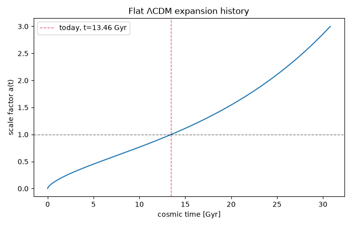
Age of the universe: 13.46 Gyr
Hubble parameter today: 70.0 km/s/Mpc

Distance-redshift relation

z = np.linspace(0.01, 5.0, 100)
d_comoving = np.array([cosmo.comoving_distance_mpc(zi) for zi in z])
d_luminosity = np.array([cosmo.luminosity_distance_mpc(zi) for zi in z])

plt.figure(figsize=(7, 4.5))
plt.plot(z, d_comoving / 1000.0, label="comoving distance")
plt.plot(z, d_luminosity / 1000.0, label="luminosity distance")
plt.xlabel("redshift z")
plt.ylabel("distance [Gpc]")
plt.title("Distance-redshift relation")
plt.legend()
plt.tight_layout()

The age of the universe across the whole density-parameter plane

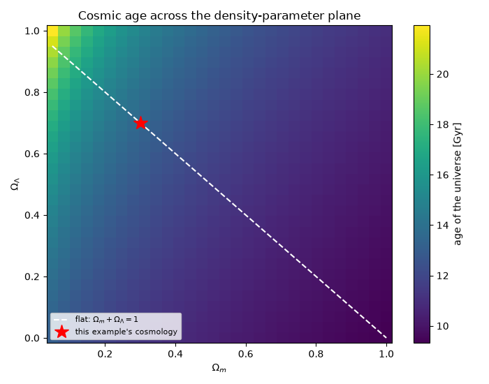
age_gyr() integrates the same Friedmann equation for any choice of \(\Omega_m, \Omega_\Lambda\) (with \(\Omega_k\) fixed so they still sum to 1 at \(a=1\)), not just the fiducial values above. Sweeping both parameters reveals the historical “age crisis” that first hinted dark energy was needed: for fixed \(\Omega_m\), a matter-only (flat) universe is younger than one with a substantial \(\Omega_\Lambda\), because more of its history was spent in the faster-decelerating, matter-dominated regime.

n_grid = 30
Om_grid = np.linspace(0.05, 1.0, n_grid)
OL_grid = np.linspace(0.0, 1.0, n_grid)
age_map = np.zeros((n_grid, n_grid))
for i, OL in enumerate(OL_grid):
    for j, Om in enumerate(Om_grid):
        age_map[i, j] = FLRWCosmology(H0=70.0, Omega_m=Om, Omega_r=9.0e-5, Omega_Lambda=OL).age_gyr(1.0)

plt.figure(figsize=(7, 5.5))
im = plt.pcolormesh(Om_grid, OL_grid, age_map, shading="auto", cmap="viridis")
plt.colorbar(im, label="age of the universe [Gyr]")
plt.plot(Om_grid, 1.0 - Om_grid, "w--", linewidth=1.5, label=r"flat: $\Omega_m+\Omega_\Lambda=1$")
plt.plot(0.3, 0.7, "r*", ms=15, label="this example's cosmology")
plt.xlabel(r"$\Omega_m$")
plt.ylabel(r"$\Omega_\Lambda$")
plt.title("Cosmic age across the density-parameter plane")
plt.legend(loc="lower left", fontsize=8)
plt.tight_layout()
plt.show()