Einstein rings, multiple images, and microlensing

When a point source, a point (or compact) lens of mass \(M\), and an observer are exactly aligned, gravitational lensing bends the source’s light into a complete ring of angular radius

\[\theta_E = \sqrt{\frac{4M D_{LS}}{D_L D_S}}\]

– an Einstein ring, predicted by Einstein in 1936 and finally imaged around a galaxy-scale lens in 1988, where \(D_L\), \(D_S\), and \(D_{LS}\) are the observer-lens, observer-source, and lens-source distances. For any imperfect alignment (true angular source offset \(\beta \ne 0\)), the thin-lens equation \(\beta = \theta - \theta_E^2/\theta\) splits the source into two images at

\[\theta_\pm = \frac{\beta \pm \sqrt{\beta^2 + 4\theta_E^2}}{2}\]

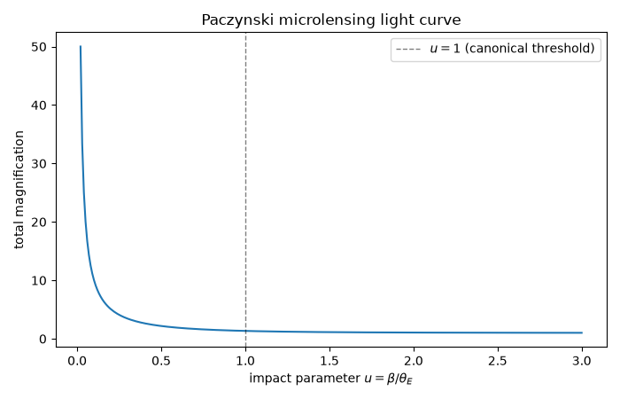
with a combined magnification (Paczynski 1986), in terms of \(u = \beta/\theta_E\),

\[\mu_\pm = \frac{1}{2}\left[\frac{u^2+2}{u\sqrt{u^2+4}} \pm 1\right]\]

that can grow dramatically as the alignment tightens (\(u \to 0\)) – the basis of gravitational microlensing surveys, used to detect exoplanets and dark, compact objects that emit no light of their own.

import matplotlib.pyplot as plt
import numpy as np

from physicskit.relativity.chapters.lensing import PointMassLens, exact_deflection_angle
from physicskit.relativity.chapters.schwarzschild import SchwarzschildBlackHole

Image positions as the source moves across the lens

lens = PointMassLens(M=1.0, D_L=1000.0, D_S=2000.0)
theta_E = lens.einstein_angle()
print(f"Einstein ring angular radius: {theta_E:.5f} rad ({np.degrees(theta_E) * 3600:.2f} arcsec-equivalent)")

beta_values = np.linspace(-4.0 * theta_E, 4.0 * theta_E, 200)
theta_plus, theta_minus = lens.image_angles(beta_values)

fig, ax = plt.subplots(figsize=(7, 5))
ax.plot(beta_values / theta_E, theta_plus / theta_E, label=r"$\theta_+$ (primary image)")
ax.plot(beta_values / theta_E, theta_minus / theta_E, label=r"$\theta_-$ (secondary image)")
ax.plot(
    beta_values / theta_E,
    beta_values / theta_E,
    "k--",
    linewidth=1,
    alpha=0.5,
    label="unlensed source",
)
ax.axhline(0, color="gray", linewidth=0.5)
ax.set_xlabel(r"source position $\beta / \theta_E$")
ax.set_ylabel(r"image position $\theta / \theta_E$")
ax.set_title("Point-lens image positions")
ax.legend()
plt.tight_layout()

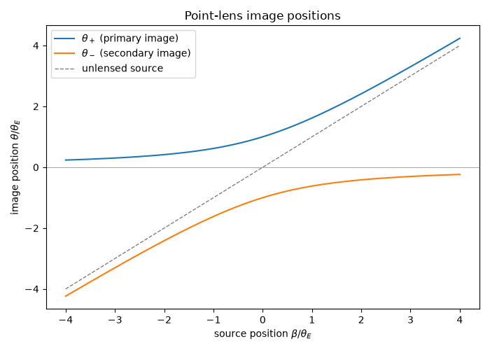
Einstein ring angular radius: 0.04472 rad (9224.44 arcsec-equivalent)

The microlensing magnification light curve

u_values = np.linspace(0.02, 3.0, 300)
totals = np.array([lens.magnification(u * theta_E)[2] for u in u_values])

plt.figure(figsize=(7, 4.5))
plt.plot(u_values, totals)
plt.axvline(1.0, color="k", linestyle="--", linewidth=1, alpha=0.5, label="$u=1$ (canonical threshold)")
plt.xlabel(r"impact parameter $u = \beta/\theta_E$")
plt.ylabel("total magnification")
plt.title("Paczynski microlensing light curve")
plt.legend()
plt.tight_layout()

Strong-field correction: the exact deflection angle vs. the weak-field 4M/b

PointMassLens uses the weak-field deflection \(\hat\alpha(b) \approx 4M/b\), valid for \(b \gg M\). As the impact parameter shrinks toward the photon sphere, the true deflection (found here by numerically integrating the actual null geodesic) grows well beyond this linear estimate.

bh = SchwarzschildBlackHole(M=1.0)
impact_params = np.array([200.0, 50.0, 20.0, 15.0])
for b in impact_params:
    exact = exact_deflection_angle(bh, b, n_steps=600000)
    weak = bh.light_deflection_angle(b)
    print(f"b={b:>6.1f}M: exact={exact:.4f} rad, weak-field 4M/b={weak:.4f} rad")

b= 200.0M: exact=0.0188 rad, weak-field 4M/b=0.0200 rad
b=  50.0M: exact=0.0847 rad, weak-field 4M/b=0.0800 rad
b=  20.0M: exact=0.2360 rad, weak-field 4M/b=0.2000 rad
b=  15.0M: exact=0.3363 rad, weak-field 4M/b=0.2667 rad

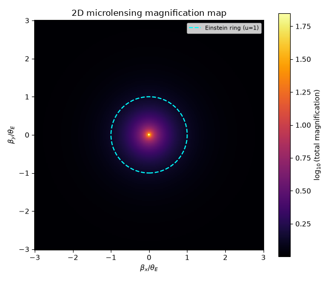
The full 2D microlensing magnification map

The light curve above only scans one straight-line path of the source behind the lens. Because PointMassLens.magnification() depends only on the angular separation \(\beta\), evaluating it over an entire 2D grid of source offsets \((\beta_x, \beta_y)\) – rather than along a single 1D track – traces out the full magnification map any real microlensing survey scans across as source and lens drift past each other, with the Einstein ring (\(u=\beta/\theta_E=1\)) as its natural scale.

n_grid = 300
extent = 3.0 * theta_E
bx = np.linspace(-extent, extent, n_grid)
by = np.linspace(-extent, extent, n_grid)
BX, BY = np.meshgrid(bx, by)
beta_mag = np.sqrt(BX**2 + BY**2)
beta_mag[beta_mag < 1.0e-6 * theta_E] = 1.0e-6 * theta_E  # avoid the beta=0 singularity
_, _, total_mag = lens.magnification(beta_mag)

fig, ax = plt.subplots(figsize=(6.5, 5.5))
im = ax.pcolormesh(bx / theta_E, by / theta_E, np.log10(total_mag), shading="auto", cmap="inferno")
plt.colorbar(im, ax=ax, label=r"$\log_{10}$(total magnification)")
ring = plt.Circle((0, 0), 1.0, fill=False, color="cyan", linestyle="--", linewidth=1.5)
ax.add_patch(ring)
ax.plot([], [], color="cyan", linestyle="--", label="Einstein ring (u=1)")
ax.set_aspect("equal")
ax.set_xlabel(r"$\beta_x / \theta_E$")
ax.set_ylabel(r"$\beta_y / \theta_E$")
ax.set_title("2D microlensing magnification map")
ax.legend(loc="upper right", fontsize=8)
plt.tight_layout()
plt.show()