The neutron star maximum mass: solving the TOV equations

Oppenheimer and Volkoff’s 1939 relativistic generalization of hydrostatic equilibrium predicts something Newtonian gravity cannot: a maximum possible mass for a neutron star. The star’s matter is modeled as a polytrope, \(P = K\rho_0^\Gamma\), relating pressure to rest-mass density, with total energy density (rest mass plus internal energy) \(\varepsilon = \rho_0 + P/(\Gamma-1)\). Enclosed mass \(m(r)\) and pressure \(P(r)\) then obey the Tolman-Oppenheimer-Volkoff equations

\[\frac{dm}{dr} = 4\pi r^2 \varepsilon, \qquad \frac{dP}{dr} = -\frac{(\varepsilon + P)\left(m + 4\pi r^3 P\right)}{r(r - 2m)}\]

integrated outward from the center to the surface where \(P \to 0\). Below the maximum mass, degenerate neutron pressure can hold the star up against its own gravity indefinitely; add matter beyond it, and no pressure can resist collapse – the star must become a black hole. This example integrates the TOV equations for a range of central densities \(\rho_0(0)\), tracing out the mass-radius relation and its characteristic maximum-mass turning point, for the classic \(K=100\), \(\Gamma=2\) polytrope benchmark used throughout the numerical relativity literature.

import matplotlib.pyplot as plt
import numpy as np

from physicskit.relativity.chapters.neutron_star import NeutronStar

The mass-radius relation and its maximum-mass turning point

star = NeutronStar(K=100.0, Gamma=2.0)
central_densities = np.logspace(-3.3, -2.2, 40)
masses, radii = star.mass_radius_curve(central_densities)

idx_max = np.argmax(masses)
print(f"Maximum mass: M={masses[idx_max]:.3f}, R={radii[idx_max]:.3f}, at rho_c={central_densities[idx_max]:.5f}")

fig, axes = plt.subplots(1, 2, figsize=(12, 4.5))
axes[0].plot(radii, masses, marker=".", ms=3)
axes[0].plot(radii[idx_max], masses[idx_max], "r*", ms=15, label="maximum mass")
axes[0].set_xlabel("radius R [M_sun-equivalent length]")
axes[0].set_ylabel("mass M")
axes[0].set_title("Mass-radius relation")
axes[0].legend()

axes[1].plot(central_densities, masses, marker=".", ms=3)
axes[1].axvline(central_densities[idx_max], color="r", linestyle="--", linewidth=1)
axes[1].set_xscale("log")
axes[1].set_xlabel(r"central density $\rho_c$")
axes[1].set_ylabel("mass M")
axes[1].set_title("Beyond the maximum, higher density means LESS mass\n(unstable branch)")
plt.tight_layout()

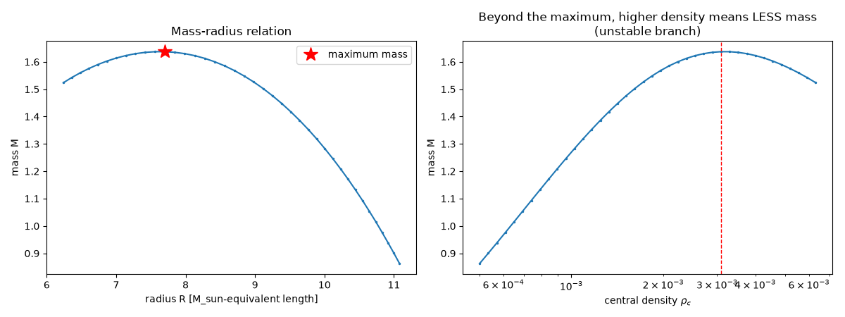
Maximum mass: M=1.637, R=7.701, at rho_c=0.00309

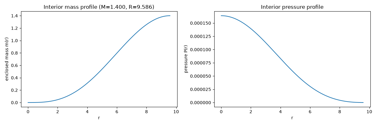
Interior structure profile of one representative star

M, R, sol = star.solve(central_density=1.28e-3)
r_grid = np.linspace(1.0e-6, R, 300)
m_profile, P_profile = sol.sol(r_grid)
P_profile = np.clip(P_profile, 0.0, None)

fig, axes = plt.subplots(1, 2, figsize=(12, 4))
axes[0].plot(r_grid, m_profile)
axes[0].set_xlabel("r")
axes[0].set_ylabel("enclosed mass m(r)")
axes[0].set_title(f"Interior mass profile (M={M:.3f}, R={R:.3f})")

axes[1].plot(r_grid, P_profile)
axes[1].set_xlabel("r")
axes[1].set_ylabel("pressure P(r)")
axes[1].set_title("Interior pressure profile")
plt.tight_layout()
plt.show()