Kruskal-Szekeres and Penrose-Carter diagrams: the true shape of spacetime

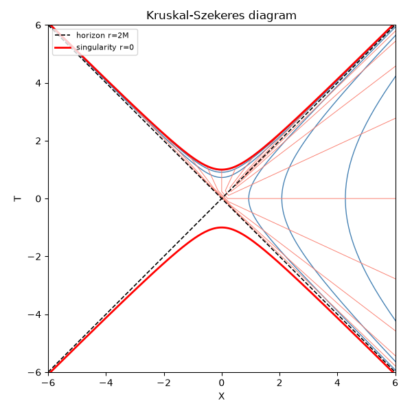
Schwarzschild coordinates \((t, r)\) blow up at the horizon \(r=2M\) – a coordinate artifact, since nothing physical happens there (a free-falling observer notices nothing special crossing it). Kruskal and Szekeres found coordinates \((X, T)\) that are perfectly smooth across the horizon: in the exterior (\(r>2M\)),

\[X = \sqrt{r/2M - 1}\, e^{r/4M} \cosh(t/4M), \qquad T = \sqrt{r/2M - 1}\, e^{r/4M} \sinh(t/4M)\]

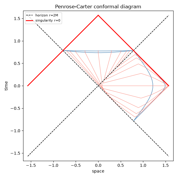
(with \(\sinh\) and \(\cosh\) swapping roles inside the horizon), so that light rays always travel at \(\pm 45^\circ\) and the horizon itself maps to the lines \(X=\pm T\). These coordinates reveal a startling fact: the maximally extended spacetime contains two separate asymptotically flat exterior regions, joined by a non-traversable “Einstein-Rosen bridge.” Compactifying further – applying \(\arctan\) to the null combinations \(u=T-X\), \(v=T+X\) – gives the Penrose-Carter diagram, bringing the entire infinite spacetime, including future and past null infinity, into one finite diagram while preserving the \(\pm 45^\circ\) light cones, making the whole causal structure visible at a glance.

import matplotlib.pyplot as plt

from physicskit.relativity.visualizers.spacetime_diagrams import plot_kruskal_diagram, plot_penrose_diagram

Kruskal-Szekeres diagram

fig, ax = plt.subplots(figsize=(6, 6))
plot_kruskal_diagram(M=1.0, ax=ax)
plt.tight_layout()

Penrose-Carter conformal diagram

fig, ax = plt.subplots(figsize=(6, 6))
plot_penrose_diagram(M=1.0, ax=ax)
plt.tight_layout()
plt.show()