Embedded Ensembles: the Two-Body Random Ensemble Is Gaussian, not Semicircle

Reproduces the celebrated French-Wong / Bohigas-Flores result: embedding a random two-body interaction into the many-particle Fock space (the Two-Body Random Ensemble, TBRE) produces correlated many-body matrix elements whose density of states approaches a GAUSSIAN, not Wigner’s semicircle, unlike an ordinary GOE Hamiltonian of the same dimension built from independent entries.

References: J. B. French, S. S. M. Wong, Phys. Lett. B 33 (1970) 449. O. Bohigas, J. Flores, Phys. Lett. B 34 (1971) 261. K. K. Mon, J. B. French, Ann. Phys. 95 (1975) 90.

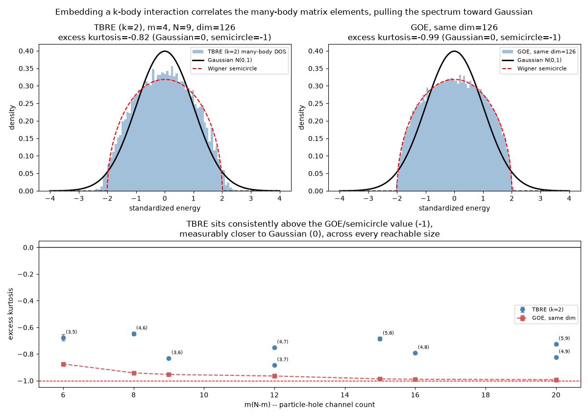
A caveat that matters for reading the figure below: the Gaussian result is an ASYMPTOTIC statement, m, N -> infinity at fixed interaction rank k = 2. Exact diagonalization costs O(C(N,k)^2 * 2^(3N)) (see physicskit.rmt.ensembles.embedded), exponential in N, so this script cannot reach system sizes where the many-body density of states actually looks Gaussian by eye – at every size reachable here (top panels), the TBRE histogram is still visibly much closer to the semicircle than to a Gaussian, just like the ordinary GOE of the same dimension next to it. What IS robustly measurable at these small sizes is the excess kurtosis (0 for a Gaussian, -1 for the semicircle): the bottom panel sweeps several (m, N) pairs and shows the TBRE value sitting consistently, measurably above its same-dimension GOE reference, even though neither histogram is visually distinguishable from the other. That gap – not the shape of a single histogram – is the honest, reachable signature of the k-body correlation structure driving the many-body spectrum away from the semicircle. (The two original papers established the full asymptotic Gaussian shape using analytic combinatorial moment formulas, not brute force diagonalization, for exactly this reason.)

import matplotlib.pyplot as plt
import numpy as np
from scipy.stats import kurtosis

import physicskit.rmt as rmt

SEED = 2026

# (n_particles, n_levels, n_samples) -- sample counts are tuned so cheap
# (small-dimension) configurations get enough draws for a tight bootstrap
# error bar, while the two most expensive ones (dim=126, cost dominated by
# 2^9 x 2^9 dense operator products) stay affordable. (4, 9) is also the
# system size shown as a standalone histogram in the left panel.
CONFIGS = [
    (3, 5, 600),
    (4, 6, 600),
    (3, 6, 500),
    (4, 7, 300),
    (3, 7, 300),
    (5, 8, 120),
    (4, 8, 120),
    (5, 9, 48),
    (4, 9, 48),
]
FEATURED = (4, 9)  # shown as the left-panel histogram


def standardize(eigs: np.ndarray) -> np.ndarray:
    flat = eigs.ravel()
    return (flat - flat.mean()) / flat.std()


def bootstrap_kurtosis_se(eigenvalues: np.ndarray, n_boot: int = 200) -> float:
    """Standard error of the excess-kurtosis estimate, via bootstrap
    resampling over independent realizations (rows of ``eigenvalues``).

    Eigenvalues *within* one realization are correlated by level
    repulsion, so only resampling whole rows -- independent draws of the
    random interaction -- gives a statistically valid error bar.
    """
    rng = np.random.default_rng(0)
    n_samples = eigenvalues.shape[0]
    boots = np.empty(n_boot)
    for i in range(n_boot):
        idx = rng.integers(0, n_samples, n_samples)
        boots[i] = kurtosis(standardize(eigenvalues[idx]))
    return boots.std()


results = []  # (m, N, dim, tbre_kurt, tbre_err, goe_kurt, goe_err)
featured_spectra = None

for m, n_levels, n_samples in CONFIGS:
    tbre = rmt.ensembles.TwoBodyRandomEnsemble(n_particles=m, n_levels=n_levels, beta=1, seed=SEED)
    tbre_spectrum = tbre.sample(n_samples=n_samples)
    dim = tbre_spectrum.eigenvalues.shape[1]  # C(n_levels, m)

    # GOE sampling is cheap regardless of dim, so give it extra draws to
    # keep its error bar tight -- it is the fixed reference, not the
    # quantity under study.
    goe = rmt.ensembles.GOE(n=dim, seed=SEED)
    goe_spectrum = goe.sample(n_samples=max(n_samples, 200))

    tbre_kurt = kurtosis(standardize(tbre_spectrum.eigenvalues))
    tbre_err = bootstrap_kurtosis_se(tbre_spectrum.eigenvalues)
    goe_kurt = kurtosis(standardize(goe_spectrum.eigenvalues))
    goe_err = bootstrap_kurtosis_se(goe_spectrum.eigenvalues)
    results.append((m, n_levels, dim, tbre_kurt, tbre_err, goe_kurt, goe_err))

    if (m, n_levels) == FEATURED:
        featured_spectra = (tbre_spectrum, goe_spectrum, dim)

results.sort(key=lambda r: r[0] * (r[1] - r[0]))  # by m(N-m), the particle-hole channel count

tbre_spectrum, goe_spectrum, feat_dim = featured_spectra
tbre_std = standardize(tbre_spectrum.eigenvalues)
goe_std = standardize(goe_spectrum.eigenvalues)

x_grid = np.linspace(-4, 4, 400)
gaussian_pdf = np.exp(-(x_grid**2) / 2) / np.sqrt(2 * np.pi)
semicircle_pdf = rmt.stats.semicircle_pdf(x_grid, radius=2.0)

fig, axd = plt.subplot_mosaic(
    [["tbre", "goe"], ["kurt", "kurt"]],
    figsize=(12, 8.5),
)

feat_tbre_kurt = kurtosis(tbre_std)
feat_goe_kurt = kurtosis(goe_std)

axd["tbre"].hist(
    tbre_std,
    bins=60,
    density=True,
    alpha=0.5,
    color="steelblue",
    label="TBRE (k=2) many-body DOS",
)
axd["tbre"].plot(x_grid, gaussian_pdf, "k-", lw=2, label="Gaussian N(0,1)")
axd["tbre"].plot(x_grid, semicircle_pdf, "r--", lw=1.5, label="Wigner semicircle")
axd["tbre"].set_title(f"TBRE (k=2), m={FEATURED[0]}, N={FEATURED[1]}, dim={feat_dim}\nexcess kurtosis={feat_tbre_kurt:.2f} (Gaussian=0, semicircle=-1)")
axd["tbre"].set_xlabel("standardized energy")
axd["tbre"].set_ylabel("density")
axd["tbre"].legend(fontsize=8)

axd["goe"].hist(
    goe_std,
    bins=60,
    density=True,
    alpha=0.5,
    color="steelblue",
    label=f"GOE, same dim={feat_dim}",
)
axd["goe"].plot(x_grid, gaussian_pdf, "k-", lw=2, label="Gaussian N(0,1)")
axd["goe"].plot(x_grid, semicircle_pdf, "r--", lw=1.5, label="Wigner semicircle")
axd["goe"].set_title(f"GOE, same dim={feat_dim}\nexcess kurtosis={feat_goe_kurt:.2f} (Gaussian=0, semicircle=-1)")
axd["goe"].set_xlabel("standardized energy")
axd["goe"].set_ylabel("density")
axd["goe"].legend(fontsize=8)

sizes = np.array([m * (n_levels - m) for m, n_levels, *_ in results])
tbre_kurts = np.array([r[3] for r in results])
tbre_errs = np.array([r[4] for r in results])
goe_kurts = np.array([r[5] for r in results])
goe_errs = np.array([r[6] for r in results])

axd["kurt"].axhline(0.0, color="black", lw=1, ls="-")
axd["kurt"].axhline(-1.0, color="red", lw=1, ls="--")
axd["kurt"].errorbar(
    sizes,
    tbre_kurts,
    yerr=tbre_errs,
    fmt="o",
    color="steelblue",
    label="TBRE (k=2)",
    capsize=3,
)
axd["kurt"].errorbar(
    sizes,
    goe_kurts,
    yerr=goe_errs,
    fmt="s--",
    color="indianred",
    label="GOE, same dim",
    capsize=3,
)
for m, n_levels, _dim, tk, *_ in results:
    axd["kurt"].annotate(
        f"({m},{n_levels})",
        (m * (n_levels - m), tk),
        textcoords="offset points",
        xytext=(4, 6),
        fontsize=7,
    )
axd["kurt"].set_xlabel("m(N-m) -- particle-hole channel count")
axd["kurt"].set_ylabel("excess kurtosis")
axd["kurt"].set_title("TBRE sits consistently above the GOE/semicircle value (-1),\nmeasurably closer to Gaussian (0), across every reachable size")
axd["kurt"].legend(fontsize=8)

fig.suptitle(
    "Embedding a k-body interaction correlates the many-body matrix elements, pulling the spectrum toward Gaussian",
)
fig.tight_layout()
plt.show()

print("\n m   N  dim  TBRE kurtosis        GOE kurtosis")
for m, n_levels, dim, tk, te, gk, ge in results:
    print(f"{m:2d} {n_levels:3d} {dim:4d}  {tk:6.3f} +/- {te:.3f}   {gk:6.3f} +/- {ge:.3f}")

m   N  dim  TBRE kurtosis        GOE kurtosis
3   5   10  -0.677 +/- 0.024   -0.874 +/- 0.013
4   6   15  -0.647 +/- 0.014   -0.941 +/- 0.008
3   6   20  -0.831 +/- 0.008   -0.953 +/- 0.005
4   7   35  -0.751 +/- 0.008   -0.965 +/- 0.005
3   7   35  -0.883 +/- 0.007   -0.965 +/- 0.005
5   8   56  -0.685 +/- 0.015   -0.986 +/- 0.003
4   8   70  -0.791 +/- 0.009   -0.989 +/- 0.003
5   9  126  -0.725 +/- 0.009   -0.992 +/- 0.002
4   9  126  -0.823 +/- 0.007   -0.992 +/- 0.002

Check

At every reachable size the TBRE excess kurtosis sits well above (more than 3 standard errors) its same-dimension GOE reference, which itself approaches the semicircle’s -1.

for m, n_levels, _dim, tk, te, gk, ge in results:
    assert tk - gk > 3 * np.hypot(te, ge), (m, n_levels)
assert abs(goe_kurts[-1] + 1) < 0.02