Dyson’s Circular Ensembles: COE, CUE, CSE

Dyson’s circular ensembles are built from Haar-random unitary matrices rather than Gaussian Hermitian ones: CUE (\(\beta=2\)) is simply the eigenvalue phases of a Haar-random \(U(n)\) matrix; COE (\(\beta=1\)) uses the symmetric unitary matrix \(U = V^T V\) for \(V\) Haar-random in \(U(n)\); CSE (\(\beta=4\)) uses the self-dual unitary \(U = V^R V\) built from a Haar-random \(V \in U(2n)\) (its \(2n\) eigenvalues occur in doubly degenerate pairs, of which \(n\) distinct phases are kept). Because Haar measure is exactly rotation-invariant, the eigenvalue phases \(\theta \in [0, 2\pi)\) are, after rescaling by \(n/(2\pi)\), exactly unfolded to unit mean spacing at any finite \(n\) – no asymptotic unfolding is needed, unlike the Gaussian/Wishart ensembles.

Despite this different construction, the nearest-neighbor spacing distribution \(P(s)\) still follows the same (generalized) Wigner surmise \(P_\beta(s) = a(\beta)\, s^\beta\, e^{-b(\beta) s^2}\) at the matching Dyson index – a universality cross-check between the Gaussian and circular families.

For CUE specifically, the exact bulk two-point correlation function (the pair-correlation “R2” of the eigenphase point process) is known in closed form as a sine kernel:

\[R_2(r) = 1 - \left(\frac{\sin(\pi r)}{\pi r}\right)^2,\]

which vanishes at \(r=0\) (complete level repulsion) and approaches 1 (no correlation) for large separations \(r\), in units of the mean spacing. This example reproduces Dyson’s circular ensembles (COE, CUE, CSE): unfolded level spacing against the Wigner surmise, and CUE’s exact bulk two-point correlation function against the sine kernel.

References: F. J. Dyson, J. Math. Phys. 3 (1962) 140, 157, 166. F. Mezzadri, Notices Amer. Math. Soc. 54 (2007) 592.

Run:

python examples/paper_replications/circular_ensembles_demo.py

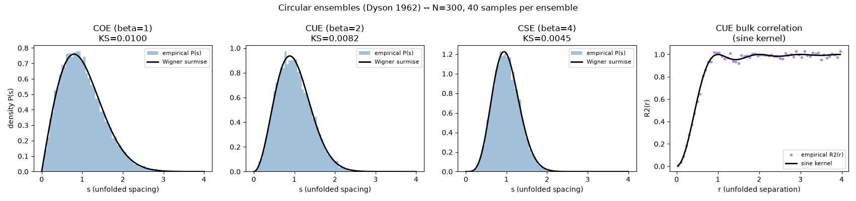
Saved circular_ensembles_replication.png

import matplotlib.pyplot as plt
import numpy as np

import physicskit.rmt as rmt

N = 300
N_SAMPLES = 40
SEED = 2026

fig, axes = plt.subplots(1, 4, figsize=(17, 4))
s_grid = np.linspace(0, 4, 400)

for col, (label, cls, beta) in enumerate(
    [("COE (beta=1)", rmt.ensembles.COE, 1), ("CUE (beta=2)", rmt.ensembles.CUE, 2), ("CSE (beta=4)", rmt.ensembles.CSE, 4)]
):
    ensemble = cls(n=N, seed=SEED)
    spectrum = ensemble.sample(n_samples=N_SAMPLES)
    spacings = rmt.stats.circular_spacings(spectrum)
    benchmark = rmt.validation.WignerSurmise(beta=beta)
    result = benchmark.validate(spacings, seed=SEED)

    ax = axes[col]
    ax.hist(spacings, bins=60, density=True, alpha=0.5, color="steelblue", label="empirical P(s)")
    ax.plot(s_grid, benchmark.theoretical_pdf(s_grid), "k-", lw=2, label="Wigner surmise")
    ax.set_title(f"{label}\nKS={result.ks_statistic:.4f}")
    ax.set_xlabel("s (unfolded spacing)")
    ax.legend(fontsize=8)

# Fourth panel: the sine kernel (CUE only -- see stats/correlations.py)
cue_ensemble = rmt.ensembles.CUE(n=400, seed=SEED)
cue_spectrum = cue_ensemble.sample(n_samples=80)
centers, estimate = rmt.stats.pair_correlation_estimate(cue_spectrum, r_max=4.0, n_bins=60)
theory_r2 = rmt.stats.sine_kernel_r2(centers)

ax = axes[3]
ax.plot(centers, estimate, "o", ms=3, color="mediumpurple", alpha=0.7, label="empirical R2(r)")
ax.plot(centers, theory_r2, "k-", lw=2, label="sine kernel")
ax.set_title("CUE bulk correlation\n(sine kernel)")
ax.set_xlabel("r (unfolded separation)")
ax.set_ylabel("R2(r)")
ax.legend(fontsize=8)

axes[0].set_ylabel("density P(s)")
fig.suptitle(
    f"Circular ensembles (Dyson 1962) -- N={N}, {N_SAMPLES} samples per ensemble",
)
fig.tight_layout()
out_path = "circular_ensembles_replication.png"
fig.savefig(out_path, dpi=150)
print(f"Saved {out_path}")