Ginibre’s Circular Law

The Ginibre ensembles GinOE (real), GinUE (complex), and GinSE (quaternion) drop the Hermitian/unitary symmetry constraint entirely: their \(n \times n\) matrices have i.i.d. Gaussian entries with no further structure, so eigenvalues are genuinely complex, spread over a two-dimensional region rather than confined to the real line or a circle. After rescaling by \(\sqrt{n}\) (Ginibre’s exact result, not just asymptotic), the eigenvalues fill the unit disk uniformly as \(n \to \infty\) – the circular law. Because a uniform density on a disk is awkward to validate directly, this example instead checks the radial marginal: integrating out the angle, the magnitude \(r = |\lambda|\) has the simple closed-form density

\[f(r) = 2r, \qquad 0 \leq r \leq 1\]

(equivalently \(F(r) = r^2\)), against which the empirical eigenvalue radii from GinOE/GinUE/GinSE are compared via a Kolmogorov-Smirnov test. GinOE and GinSE eigenvalues are not confined to the disk’s generic bulk in exactly the same way as GinUE (GinOE mixes real eigenvalues with complex-conjugate pairs; GinSE’s \(2n\) eigenvalues come in genuinely distinct conjugate pairs, not Kramers-degenerate ones), but all three share the same limiting radial law. This example reproduces Ginibre’s circular law for GinOE, GinUE, GinSE: eigenvalue scatter in the complex plane against the exact unit-disk boundary, plus the radial density check used for quantitative validation.

Reference: J. Ginibre, J. Math. Phys. 6 (1965) 440.

Run:

python examples/paper_replications/circular_law_demo.py

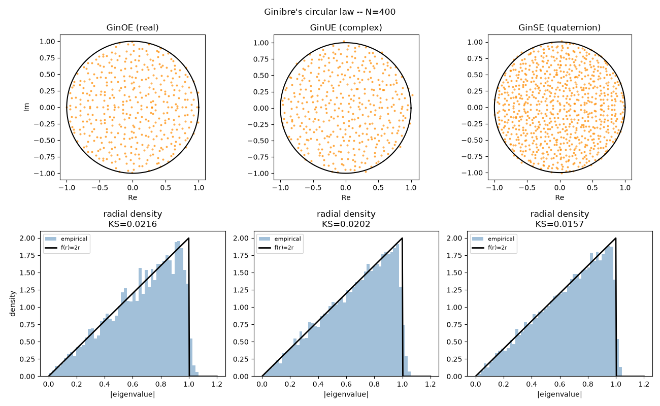
Saved circular_law_replication.png

import matplotlib.pyplot as plt
import numpy as np

import physicskit.rmt as rmt

N = 400
SEED = 2026

fig, axes = plt.subplots(2, 3, figsize=(13, 8))
theta_circle = np.linspace(0, 2 * np.pi, 300)
r_grid = np.linspace(0, 1.2, 300)

for col, (label, cls) in enumerate(
    [("GinOE (real)", rmt.ensembles.GinOE), ("GinUE (complex)", rmt.ensembles.GinUE), ("GinSE (quaternion)", rmt.ensembles.GinSE)]
):
    ensemble = cls(n=N, seed=SEED)
    spectrum = ensemble.sample(n_samples=1)
    eigs = spectrum.rescaled[0]

    ax = axes[0, col]
    ax.scatter(eigs.real, eigs.imag, s=4, alpha=0.6, color="darkorange")
    ax.plot(np.cos(theta_circle), np.sin(theta_circle), "k-", lw=1.5)
    ax.set_title(label)
    ax.set_aspect("equal")
    ax.set_xlabel("Re")

    # radial density check (pooled over more samples for a clean curve)
    spectrum_many = ensemble.sample(n_samples=20)
    radii = np.abs(spectrum_many.rescaled.ravel())
    benchmark = rmt.validation.CircularLaw()
    result = benchmark.validate(spectrum_many, seed=SEED)

    ax2 = axes[1, col]
    ax2.hist(radii, bins=50, density=True, alpha=0.5, color="steelblue", label="empirical")
    ax2.plot(r_grid, benchmark.theoretical_pdf(r_grid), "k-", lw=2, label="f(r)=2r")
    ax2.set_title(f"radial density\nKS={result.ks_statistic:.4f}")
    ax2.set_xlabel("|eigenvalue|")
    ax2.legend(fontsize=8)

axes[0, 0].set_ylabel("Im")
axes[1, 0].set_ylabel("density")
fig.suptitle(f"Ginibre's circular law -- N={N}")
fig.tight_layout()
out_path = "circular_law_replication.png"
fig.savefig(out_path, dpi=150)
print(f"Saved {out_path}")