The Two-Body Random Ensemble: Gaussian, not Semicircle

Reproduces the celebrated French-Wong / Bohigas-Flores result: embedding a random two-body interaction into the many-particle Fock space (the Two-Body Random Ensemble, TBRE) produces correlated many-body matrix elements whose density of states approaches a GAUSSIAN, not Wigner’s semicircle, unlike an ordinary GOE Hamiltonian of the same dimension built from independent entries.

References: J. B. French, S. S. M. Wong, Phys. Lett. B 33 (1970) 449. O. Bohigas, J. Flores, Phys. Lett. B 34 (1971) 261. K. K. Mon, J. B. French, Ann. Phys. 95 (1975) 90.

A caveat that matters for reading the figure below: the Gaussian result is an ASYMPTOTIC statement, m, N -> infinity at fixed interaction rank k = 2. Exact diagonalization costs O(C(N,k)^2 * 2^(3N)) (see physicskit.rmt.ensembles.embedded), exponential in N, so this script cannot reach system sizes where the many-body density of states actually looks Gaussian by eye – at every size reachable here (top panels), the TBRE histogram is still visibly much closer to the semicircle than to a Gaussian, just like the ordinary GOE of the same dimension next to it. What IS robustly measurable at these small sizes is the excess kurtosis (0 for a Gaussian, -1 for the semicircle): the bottom panel sweeps several (m, N) pairs and shows the TBRE value sitting consistently, measurably above its same-dimension GOE reference, even though neither histogram is visually distinguishable from the other. That gap – not the shape of a single histogram – is the honest, reachable signature of the k-body correlation structure driving the many-body spectrum away from the semicircle. (The two original papers established the full asymptotic Gaussian shape using analytic combinatorial moment formulas, not brute force diagonalization, for exactly this reason.)

Run:

python examples/paper_replications/embedded_ensemble_demo.py

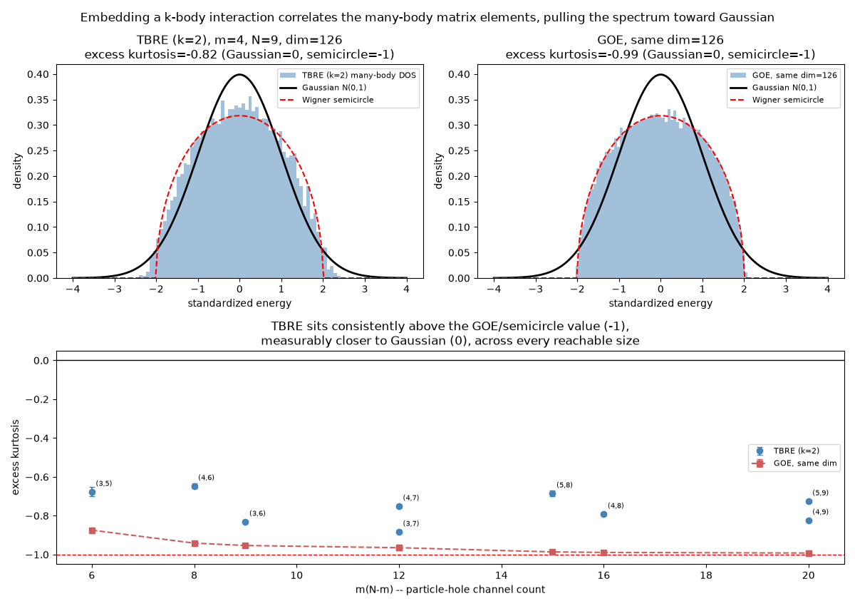
Saved embedded_ensemble_replication.png

 m   N  dim  TBRE kurtosis        GOE kurtosis
 3   5   10  -0.677 +/- 0.024   -0.874 +/- 0.013
 4   6   15  -0.647 +/- 0.014   -0.941 +/- 0.008
 3   6   20  -0.831 +/- 0.008   -0.953 +/- 0.005
 4   7   35  -0.751 +/- 0.008   -0.965 +/- 0.005
 3   7   35  -0.883 +/- 0.007   -0.965 +/- 0.005
 5   8   56  -0.685 +/- 0.015   -0.986 +/- 0.003
 4   8   70  -0.791 +/- 0.009   -0.989 +/- 0.003
 5   9  126  -0.725 +/- 0.009   -0.992 +/- 0.002
 4   9  126  -0.823 +/- 0.007   -0.992 +/- 0.002

import matplotlib.pyplot as plt
import numpy as np
from scipy.stats import kurtosis

import physicskit.rmt as rmt

SEED = 2026

# (n_particles, n_levels, n_samples) -- sample counts are tuned so cheap
# (small-dimension) configurations get enough draws for a tight bootstrap
# error bar, while the two most expensive ones (dim=126, cost dominated by
# 2^9 x 2^9 dense operator products) stay affordable. (4, 9) is also the
# system size shown as a standalone histogram in the left panel.
CONFIGS = [
    (3, 5, 600),
    (4, 6, 600),
    (3, 6, 500),
    (4, 7, 300),
    (3, 7, 300),
    (5, 8, 120),
    (4, 8, 120),
    (5, 9, 48),
    (4, 9, 48),
]
FEATURED = (4, 9)  # shown as the left-panel histogram


def standardize(eigs: np.ndarray) -> np.ndarray:
    flat = eigs.ravel()
    return (flat - flat.mean()) / flat.std()


def bootstrap_kurtosis_se(eigenvalues: np.ndarray, n_boot: int = 200) -> float:
    """Standard error of the excess-kurtosis estimate, via bootstrap
    resampling over independent realizations (rows of ``eigenvalues``).

    Eigenvalues *within* one realization are correlated by level
    repulsion, so only resampling whole rows -- independent draws of the
    random interaction -- gives a statistically valid error bar.
    """
    rng = np.random.default_rng(0)
    n_samples = eigenvalues.shape[0]
    boots = np.empty(n_boot)
    for i in range(n_boot):
        idx = rng.integers(0, n_samples, n_samples)
        boots[i] = kurtosis(standardize(eigenvalues[idx]))
    return boots.std()


results = []  # (m, N, dim, tbre_kurt, tbre_err, goe_kurt, goe_err)
featured_spectra = None

for m, n_levels, n_samples in CONFIGS:
    tbre = rmt.ensembles.TwoBodyRandomEnsemble(n_particles=m, n_levels=n_levels, beta=1, seed=SEED)
    tbre_spectrum = tbre.sample(n_samples=n_samples)
    dim = tbre_spectrum.eigenvalues.shape[1]  # C(n_levels, m)

    # GOE sampling is cheap regardless of dim, so give it extra draws to
    # keep its error bar tight -- it is the fixed reference, not the
    # quantity under study.
    goe = rmt.ensembles.GOE(n=dim, seed=SEED)
    goe_spectrum = goe.sample(n_samples=max(n_samples, 200))

    tbre_kurt = kurtosis(standardize(tbre_spectrum.eigenvalues))
    tbre_err = bootstrap_kurtosis_se(tbre_spectrum.eigenvalues)
    goe_kurt = kurtosis(standardize(goe_spectrum.eigenvalues))
    goe_err = bootstrap_kurtosis_se(goe_spectrum.eigenvalues)
    results.append((m, n_levels, dim, tbre_kurt, tbre_err, goe_kurt, goe_err))

    if (m, n_levels) == FEATURED:
        featured_spectra = (tbre_spectrum, goe_spectrum, dim)

results.sort(key=lambda r: r[0] * (r[1] - r[0]))  # by m(N-m), the particle-hole channel count

tbre_spectrum, goe_spectrum, feat_dim = featured_spectra
tbre_std = standardize(tbre_spectrum.eigenvalues)
goe_std = standardize(goe_spectrum.eigenvalues)

x_grid = np.linspace(-4, 4, 400)
gaussian_pdf = np.exp(-(x_grid**2) / 2) / np.sqrt(2 * np.pi)
semicircle_pdf = rmt.stats.semicircle_pdf(x_grid, radius=2.0)

fig, axd = plt.subplot_mosaic(
    [["tbre", "goe"], ["kurt", "kurt"]],
    figsize=(12, 8.5),
)

feat_tbre_kurt = kurtosis(tbre_std)
feat_goe_kurt = kurtosis(goe_std)

axd["tbre"].hist(
    tbre_std,
    bins=60,
    density=True,
    alpha=0.5,
    color="steelblue",
    label="TBRE (k=2) many-body DOS",
)
axd["tbre"].plot(x_grid, gaussian_pdf, "k-", lw=2, label="Gaussian N(0,1)")
axd["tbre"].plot(x_grid, semicircle_pdf, "r--", lw=1.5, label="Wigner semicircle")
axd["tbre"].set_title(f"TBRE (k=2), m={FEATURED[0]}, N={FEATURED[1]}, dim={feat_dim}\nexcess kurtosis={feat_tbre_kurt:.2f} (Gaussian=0, semicircle=-1)")
axd["tbre"].set_xlabel("standardized energy")
axd["tbre"].set_ylabel("density")
axd["tbre"].legend(fontsize=8)

axd["goe"].hist(
    goe_std,
    bins=60,
    density=True,
    alpha=0.5,
    color="steelblue",
    label=f"GOE, same dim={feat_dim}",
)
axd["goe"].plot(x_grid, gaussian_pdf, "k-", lw=2, label="Gaussian N(0,1)")
axd["goe"].plot(x_grid, semicircle_pdf, "r--", lw=1.5, label="Wigner semicircle")
axd["goe"].set_title(f"GOE, same dim={feat_dim}\nexcess kurtosis={feat_goe_kurt:.2f} (Gaussian=0, semicircle=-1)")
axd["goe"].set_xlabel("standardized energy")
axd["goe"].set_ylabel("density")
axd["goe"].legend(fontsize=8)

sizes = np.array([m * (n_levels - m) for m, n_levels, *_ in results])
tbre_kurts = np.array([r[3] for r in results])
tbre_errs = np.array([r[4] for r in results])
goe_kurts = np.array([r[5] for r in results])
goe_errs = np.array([r[6] for r in results])

axd["kurt"].axhline(0.0, color="black", lw=1, ls="-")
axd["kurt"].axhline(-1.0, color="red", lw=1, ls="--")
axd["kurt"].errorbar(
    sizes,
    tbre_kurts,
    yerr=tbre_errs,
    fmt="o",
    color="steelblue",
    label="TBRE (k=2)",
    capsize=3,
)
axd["kurt"].errorbar(
    sizes,
    goe_kurts,
    yerr=goe_errs,
    fmt="s--",
    color="indianred",
    label="GOE, same dim",
    capsize=3,
)
for m, n_levels, _dim, tk, *_ in results:
    axd["kurt"].annotate(
        f"({m},{n_levels})",
        (m * (n_levels - m), tk),
        textcoords="offset points",
        xytext=(4, 6),
        fontsize=7,
    )
axd["kurt"].set_xlabel("m(N-m) -- particle-hole channel count")
axd["kurt"].set_ylabel("excess kurtosis")
axd["kurt"].set_title("TBRE sits consistently above the GOE/semicircle value (-1),\nmeasurably closer to Gaussian (0), across every reachable size")
axd["kurt"].legend(fontsize=8)

fig.suptitle(
    "Embedding a k-body interaction correlates the many-body matrix elements, pulling the spectrum toward Gaussian",
)
fig.tight_layout()
out_path = "embedded_ensemble_replication.png"
fig.savefig(out_path, dpi=150)
print(f"Saved {out_path}")

print("\n m   N  dim  TBRE kurtosis        GOE kurtosis")
for m, n_levels, dim, tk, te, gk, ge in results:
    print(f"{m:2d} {n_levels:3d} {dim:4d}  {tk:6.3f} +/- {te:.3f}   {gk:6.3f} +/- {ge:.3f}")