Page’s Conjecture: the Average Entanglement Entropy of a Random State

A Haar-random pure state on \(\mathbb{C}^n \otimes \mathbb{C}^k\) (\(n \leq k\)), traced out over the \(k\)-dimensional subsystem, leaves an \(n\)-dimensional reduced density matrix \(\rho = A A^\dagger / \mathrm{Tr}(A A^\dagger)\) built from an \(n \times k\) complex Ginibre matrix \(A\) (the “induced measure”; \(k=n\) is the flat Hilbert-Schmidt measure on density matrices). Page’s exact result gives the average von Neumann entropy \(S = -\sum_i \lambda_i \log \lambda_i\) (in nats, \(\lambda_i\) the eigenvalues of \(\rho\)) of this random reduced state, for any finite \(n, k\):

\[\langle S \rangle = \psi(nk+1) - \psi(k+1) - \frac{n-1}{2k},\]

where \(\psi\) is the digamma function. This is an exact finite-dimension result, not an asymptotic approximation. This example reproduces Page’s (1993) exact average von Neumann entropy for the reduced density matrix of a Haar-random bipartite pure state on \(\mathbb{C}^n \otimes \mathbb{C}^k\). Two views of the same formula: the classic “Page curve” (entropy rising, then turning over, as the traced-out subsystem grows past the retained one – the black-hole-evaporation analogue), and the subsystem’s entropy approaching the maximum \(\log n\) as its environment grows.

Reference: D. N. Page, Phys. Rev. Lett. 71 (1993) 1291.

Run:

python examples/paper_replications/page_curve_demo.py

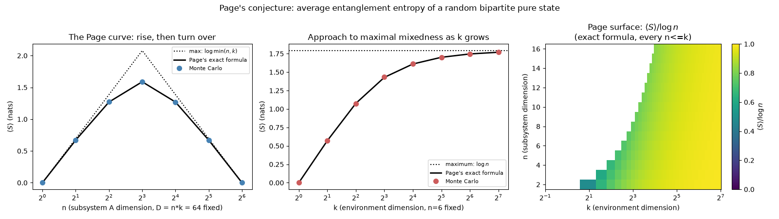
Saved page_curve_replication.png

import matplotlib.pyplot as plt
import numpy as np

import physicskit.rmt as rmt

N_SAMPLES = 300
SEED = 2026

fig, axes = plt.subplots(1, 3, figsize=(16, 4.5))

# --- Panel 1: the Page curve -- fixed total dimension D = n * k ---
D = 64
n_values = [1, 2, 4, 8, 16, 32, 64]

empirical = []
theory = []
max_entropy = []
for n_dim in n_values:
    k_dim = D // n_dim
    ensemble = rmt.ensembles.InducedMeasureEnsemble(n=n_dim, k=k_dim, seed=SEED)
    spectrum = ensemble.sample(n_samples=N_SAMPLES)
    entropies = [rmt.stats.von_neumann_entropy(row) for row in spectrum.eigenvalues]
    empirical.append(np.mean(entropies))
    theory.append(rmt.stats.page_curve_average_entropy(min(n_dim, k_dim), max(n_dim, k_dim)))
    max_entropy.append(np.log(min(n_dim, k_dim)))

ax = axes[0]
ax.plot(n_values, max_entropy, "k:", lw=1.5, label=r"max: $\log \min(n,k)$")
ax.plot(n_values, theory, "k-", lw=2, label="Page's exact formula")
ax.plot(n_values, empirical, "o", color="steelblue", ms=7, label="Monte Carlo")
ax.set_xscale("log", base=2)
ax.set_xlabel(f"n (subsystem A dimension, D = n*k = {D} fixed)")
ax.set_ylabel(r"$\langle S \rangle$ (nats)")
ax.set_title("The Page curve: rise, then turn over")
ax.legend(fontsize=8)

# --- Panel 2: fixed subsystem, growing environment -> maximally mixed ---
n_fixed = 6
k_values = [1, 2, 4, 8, 16, 32, 64, 128]

empirical2 = []
theory2 = []
for k_dim in k_values:
    ensemble = rmt.ensembles.InducedMeasureEnsemble(n=n_fixed, k=k_dim, seed=SEED + 1)
    spectrum = ensemble.sample(n_samples=N_SAMPLES)
    entropies = [rmt.stats.von_neumann_entropy(row) for row in spectrum.eigenvalues]
    empirical2.append(np.mean(entropies))
    # Page's formula assumes its first argument is the SMALLER dimension
    # (n <= k); for k_dim < n_fixed, S_A = S_B still holds exactly (the
    # global state is pure), so swap arguments rather than violate that.
    theory2.append(rmt.stats.page_curve_average_entropy(min(n_fixed, k_dim), max(n_fixed, k_dim)))

ax = axes[1]
ax.axhline(np.log(n_fixed), color="k", ls=":", lw=1.5, label=r"maximum: $\log n$")
ax.plot(k_values, theory2, "k-", lw=2, label="Page's exact formula")
ax.plot(k_values, empirical2, "o", color="indianred", ms=7, label="Monte Carlo")
ax.set_xscale("log", base=2)
ax.set_xlabel(f"k (environment dimension, n={n_fixed} fixed)")
ax.set_ylabel(r"$\langle S \rangle$ (nats)")
ax.set_title("Approach to maximal mixedness as k grows")
ax.legend(fontsize=8)

# --- Panel 3: the full (n, k) Page surface ---
# Panels 1-2 are each a single 1D slice (fixed D=n*k, then fixed n)
# through Page's exact formula; this shows the whole 2-parameter
# surface, as the fraction of maximal entropy S/log(n) reached, over
# every (n, k) pair with n <= k (the formula's domain of validity).
n_page = np.arange(2, 17)  # n=1 excluded: log(1)=0 (a 1-dim subsystem is always pure, S=0 trivially)
k_page = np.arange(1, 129)
page_fraction = np.full((len(n_page), len(k_page)), np.nan)
for i, n_dim in enumerate(n_page):
    for j, k_dim in enumerate(k_page):
        if k_dim < n_dim:
            continue
        page_fraction[i, j] = rmt.stats.page_curve_average_entropy(int(n_dim), int(k_dim)) / np.log(n_dim)

ax = axes[2]
im = ax.pcolormesh(k_page, n_page, page_fraction, cmap="viridis", vmin=0.0, vmax=1.0, shading="nearest")
ax.set_xscale("log", base=2)
ax.set_xlabel("k (environment dimension)")
ax.set_ylabel("n (subsystem dimension)")
ax.set_title(r"Page surface: $\langle S \rangle / \log n$" + "\n(exact formula, every n<=k)")
fig.colorbar(im, ax=ax, label=r"$\langle S \rangle / \log n$")

fig.suptitle(
    "Page's conjecture: average entanglement entropy of a random bipartite pure state",
)
fig.tight_layout()
out_path = "page_curve_replication.png"
fig.savefig(out_path, dpi=150)
print(f"Saved {out_path}")