The Berry-Tabor Poisson Baseline

The Berry-Tabor conjecture holds that a classically integrable system’s quantum energy levels, having no level repulsion mechanism to correlate them, behave locally like an uncorrelated (Poisson) point process – in sharp contrast to a chaotic system’s GOE/GUE/GSE-type statistics. PoissonEnsemble realizes this null model directly (independent, uniformly spaced levels with no repulsion built in). Two statistics distinguish the two regimes:

The nearest-neighbor spacing density is exponential for Poisson,

\[P(s) = e^{-s},\]

with no suppression of small spacings (no level repulsion), versus the Wigner surmise’s \(P(s) \sim s^\beta e^{-b s^2}\) for GOE/GUE/GSE, which vanishes at \(s=0\).

The number variance \(\Sigma^2(L)\) – the variance of the eigenvalue count in a randomly placed interval of (unfolded) length \(L\) – grows linearly for an uncorrelated sequence,

\[\Sigma^2_{\text{Poisson}}(L) = L,\]

while level repulsion makes the Gaussian ensembles’ spectra far more rigid: \(\Sigma^2_\beta(L)\) grows only logarithmically with \(L\) (Dyson-Mehta 1963),

\[\Sigma^2_\beta(L) = \frac{2}{\beta \pi^2}\ln L + K_\beta + O(1/L).\]

This example reproduces the Berry-Tabor null model: a classically integrable system’s level statistics are locally indistinguishable from an uncorrelated (Poisson) point process – no level repulsion at small spacing, and a number variance Sigma^2(L) that grows linearly with L, in sharp contrast to GOE/GUE/GSE’s logarithmically rigid, repulsive statistics.

Reference: M. V. Berry, M. Tabor, Proc. R. Soc. Lond. A 356 (1977) 375.

Run:

python examples/paper_replications/poisson_berry_tabor_demo.py

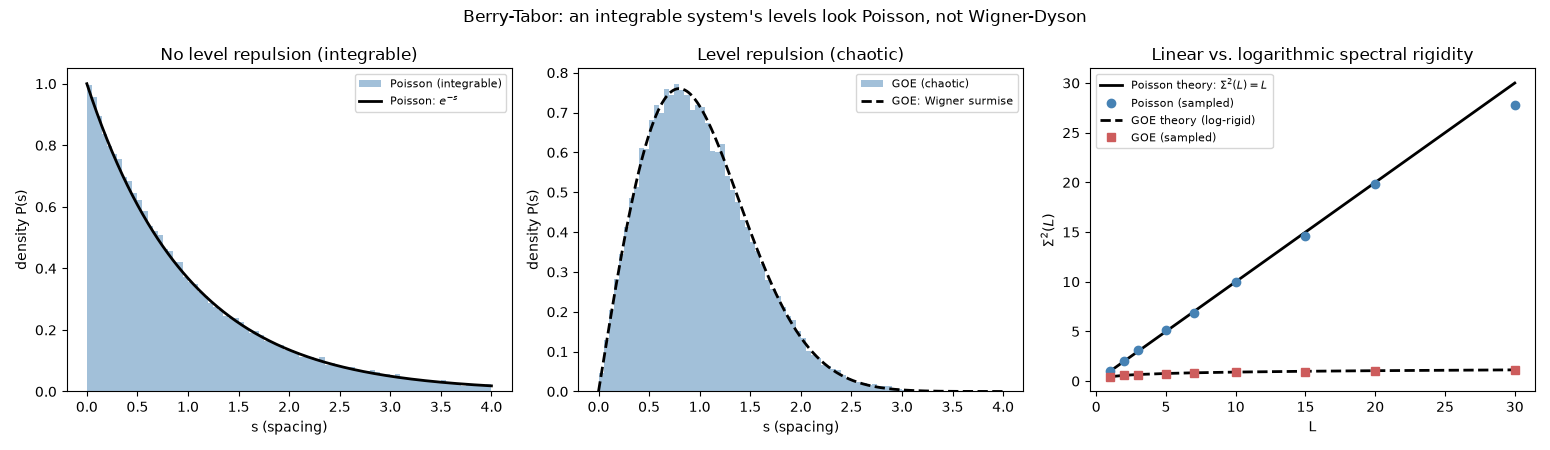
Saved poisson_berry_tabor_replication.png

import matplotlib.pyplot as plt
import numpy as np

import physicskit.rmt as rmt

N_POISSON = 3000
N_GOE = 3000
N_SAMPLES = 20
SEED = 2026

poisson_ens = rmt.ensembles.PoissonEnsemble(n=N_POISSON, seed=SEED)
poisson_spectrum = poisson_ens.sample(n_samples=N_SAMPLES)

goe_ens = rmt.ensembles.GOE(n=N_GOE, seed=SEED)
goe_spectrum = goe_ens.sample(n_samples=N_SAMPLES)

fig, axes = plt.subplots(1, 3, figsize=(15.5, 4.5))

# --- Panels 1-2: spacing distributions -- no repulsion vs. repulsion ---
poisson_spacings = np.concatenate([np.diff(row) for row in poisson_spectrum.eigenvalues])
goe_spacings = rmt.stats.nearest_neighbor_spacings(goe_spectrum, rmt.stats.semicircle_cdf)

s_grid = np.linspace(0, 4, 400)

ax = axes[0]
ax.hist(poisson_spacings, bins=80, density=True, range=(0, 4), alpha=0.5, color="steelblue", label="Poisson (integrable)")
ax.plot(s_grid, np.exp(-s_grid), "k-", lw=2, label=r"Poisson: $e^{-s}$")
ax.set_xlabel("s (spacing)")
ax.set_ylabel("density P(s)")
ax.set_title("No level repulsion (integrable)")
ax.legend(fontsize=8)

ax = axes[1]
ax.hist(goe_spacings, bins=80, density=True, range=(0, 4), alpha=0.5, color="steelblue", label="GOE (chaotic)")
ax.plot(s_grid, rmt.stats.wigner_surmise_pdf(s_grid, beta=1), "k--", lw=2, label="GOE: Wigner surmise")
ax.set_xlabel("s (spacing)")
ax.set_ylabel("density P(s)")
ax.set_title("Level repulsion (chaotic)")
ax.legend(fontsize=8)

# --- Panel 3: number variance -- linear vs. logarithmic rigidity ---
l_values = np.array([1, 2, 3, 5, 7, 10, 15, 20, 30])
rng = np.random.default_rng(SEED + 1)

poisson_empirical = []
for length in l_values:
    counts = []
    for row in poisson_spectrum.eigenvalues:
        lo, hi = row[0], row[-1]
        starts = rng.uniform(lo, hi - length, size=200)
        counts.extend(np.sum((row >= s) & (row < s + length)) for s in starts)
    poisson_empirical.append(np.var(counts))
poisson_empirical = np.array(poisson_empirical)

goe_empirical = rmt.stats.number_variance_empirical(
    goe_spectrum,
    rmt.stats.semicircle_cdf,
    l_values,
    n_windows=200,
    seed=SEED + 2,
)

ax = axes[2]
ax.plot(l_values, rmt.stats.number_variance_poisson(l_values), "k-", lw=2, label=r"Poisson theory: $\Sigma^2(L) = L$")
ax.plot(l_values, poisson_empirical, "o", color="steelblue", label="Poisson (sampled)")
ax.plot(l_values, rmt.stats.number_variance_theory(l_values, beta=1), "k--", lw=2, label="GOE theory (log-rigid)")
ax.plot(l_values, goe_empirical, "s", color="indianred", label="GOE (sampled)")
ax.set_xlabel("L")
ax.set_ylabel(r"$\Sigma^2(L)$")
ax.set_title("Linear vs. logarithmic spectral rigidity")
ax.legend(fontsize=8)

fig.suptitle(
    "Berry-Tabor: an integrable system's levels look Poisson, not Wigner-Dyson",
)
fig.tight_layout()
out_path = "poisson_berry_tabor_replication.png"
fig.savefig(out_path, dpi=150)
print(f"Saved {out_path}")