PT-Symmetry Breaking in Pseudo-Hermitian Ensembles

Bender and Boettcher observed that certain non-Hermitian Hamiltonians with PT (parity-time) symmetry can nonetheless have entirely real spectra. This ensemble realizes the equivalent condition of pseudo-Hermiticity, \(P H P^{-1} = H^\dagger\) for a fixed Hermitian involution \(P = \mathrm{diag}(I_p, -I_q)\) (\(n=p+q\)). Writing \(H\) in the matching \(2\times 2\) block form

\[\begin{split}H = \begin{pmatrix} A & B \\ -B^\dagger & D \end{pmatrix},\end{split}\]

pseudo-Hermiticity forces \(A = A^\dagger\) (\(p \times p\)), \(D = D^\dagger\) (\(q \times q\)) – independent GOE/GUE-type Hermitian blocks – while the off-diagonal (coupling) block \(B\) is an independent Ginibre-type \(p \times q\) block scaled by the non-Hermiticity strength \(g\). At \(g=0\), \(H\) is block-diagonal and trivially has a real spectrum (the “unbroken” PT-symmetric phase); since \(H\) is always similar to \(H^\dagger\), its eigenvalues remain closed under complex conjugation for any \(g\), either real or in exact complex-conjugate pairs. As \(g\) grows, an increasing fraction of eigenvalues collide (an “exceptional point”, where eigenvectors also coalesce) and split off the real axis as conjugate pairs – the PT-symmetry-breaking transition.

This example reproduces the PT-symmetry-breaking transition: the fraction of real eigenvalues of a pseudo-Hermitian ensemble drops from 1 (fully real, “unbroken” PT symmetry) toward 0 as the non-Hermiticity/coupling strength g increases.

Reference: C. M. Bender, S. Boettcher, Phys. Rev. Lett. 80 (1998) 5243.

Run:

python examples/paper_replications/pt_symmetric_demo.py

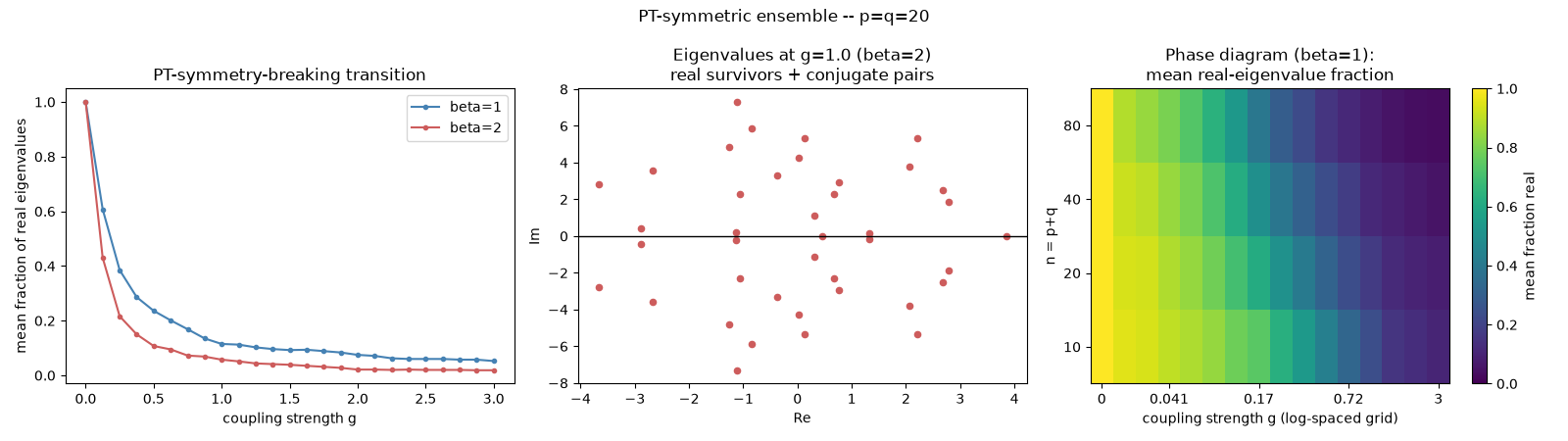
Saved pt_symmetric_replication.png

import matplotlib.pyplot as plt
import numpy as np

import physicskit.rmt as rmt

P = Q = 20
N_SAMPLES = 40
SEED = 2026

fig, axes = plt.subplots(1, 3, figsize=(16, 4.5))

g_values = np.linspace(0.0, 3.0, 25)
for beta, color in [(1, "steelblue"), (2, "indianred")]:
    fractions = []
    for g in g_values:
        ensemble = rmt.ensembles.PTSymmetricEnsemble(p=P, q=Q, g=g, beta=beta, seed=SEED)
        spectrum = ensemble.sample(n_samples=N_SAMPLES)
        fractions.append(rmt.stats.real_eigenvalue_fraction(spectrum.eigenvalues).mean())
    axes[0].plot(g_values, fractions, "o-", ms=3, color=color, label=f"beta={beta}")

axes[0].set_xlabel("coupling strength g")
axes[0].set_ylabel("mean fraction of real eigenvalues")
axes[0].set_title("PT-symmetry-breaking transition")
axes[0].legend()

# Eigenvalue scatter at a representative g, showing the real-axis
# survivors and the complex-conjugate pairs that have already split off.
ensemble = rmt.ensembles.PTSymmetricEnsemble(p=P, q=Q, g=1.0, beta=2, seed=SEED)
spectrum = ensemble.sample(n_samples=1)
eigs = spectrum.eigenvalues[0]
axes[1].scatter(eigs.real, eigs.imag, s=20, color="indianred")
axes[1].axhline(0.0, color="k", lw=1)
axes[1].set_xlabel("Re")
axes[1].set_ylabel("Im")
axes[1].set_title("Eigenvalues at g=1.0 (beta=2)\nreal survivors + conjugate pairs")

# --- Panel 3: phase diagram over (g, system size) ---
# Panel 1 fixes n=p+q=40 and only varies g; the transition itself shifts
# with system size (a larger ensemble has more real-eigenvalue pairs
# that can collide), so a 2D map of the same real_eigenvalue_fraction
# statistic over BOTH g and n resolves that size-dependence directly,
# rather than a single 1D slice through it.
g_grid_2d = np.concatenate([[0.0], np.geomspace(0.02, 3.0, 15)])
n_half_values = [5, 10, 20, 40]
fraction_grid = np.empty((len(n_half_values), len(g_grid_2d)))
for row, half in enumerate(n_half_values):
    for col, g in enumerate(g_grid_2d):
        # beta=1 (GOE-type blocks): the slower of the two transitions in
        # panel 1, giving better resolution across this g range than
        # beta=2's much sharper drop.
        ensemble = rmt.ensembles.PTSymmetricEnsemble(p=half, q=half, g=float(g), beta=1, seed=SEED)
        spectrum = ensemble.sample(n_samples=N_SAMPLES)
        fraction_grid[row, col] = rmt.stats.real_eigenvalue_fraction(spectrum.eigenvalues).mean()

ax = axes[2]
im = ax.imshow(fraction_grid, aspect="auto", origin="lower", cmap="viridis", vmin=0.0, vmax=1.0)
ax.set_yticks(range(len(n_half_values)))
ax.set_yticklabels([f"{2 * h}" for h in n_half_values])
tick_idx = [0, 3, 7, 11, 15]
ax.set_xticks(tick_idx)
ax.set_xticklabels([f"{g_grid_2d[i]:.2g}" for i in tick_idx])
ax.set_xlabel("coupling strength g (log-spaced grid)")
ax.set_ylabel("n = p+q")
ax.set_title("Phase diagram (beta=1):\nmean real-eigenvalue fraction")
fig.colorbar(im, ax=ax, label="mean fraction real")

fig.suptitle(f"PT-symmetric ensemble -- p=q={P}")
fig.tight_layout()
out_path = "pt_symmetric_replication.png"
fig.savefig(out_path, dpi=150)
print(f"Saved {out_path}")