Spectral Rigidity and Universality

Beyond nearest-neighbor spacing, the number variance \(\Sigma^2(L)\) – the variance of the eigenvalue count in a randomly placed window of (unfolded) length \(L\) – probes longer-range spectral correlations. An uncorrelated (Poisson) sequence has \(\Sigma^2(L) = L\); level repulsion makes the Gaussian ensembles’ spectra far more rigid, with only logarithmic growth (Dyson-Mehta 1963):

\[\Sigma^2_\beta(L) = \frac{2}{\beta \pi^2}\ln L + K_\beta + O(1/L).\]

Separately, this example also demonstrates universality: the limiting eigenvalue density of a Wigner-type ensemble depends only on the entries’ mean and variance, not their detailed distribution. Random symmetric matrices built from uniform, Rademacher (\(\pm 1\)), or exponential entries – after the same \(\sqrt{N}\) rescaling – all converge to the same Wigner semicircle law.

This example reproduces the Dyson-Mehta number variance \(\Sigma^2(L)\) for GOE/GUE/GSE vs. the Poisson (uncorrelated) baseline, and demonstrates universality: GUE-type spacing statistics from three very different entry distributions (uniform, Rademacher, exponential).

References: F. J. Dyson, M. L. Mehta, J. Math. Phys. 4 (1963) 701.

Run:

python examples/paper_replications/rigidity_universality_demo.py

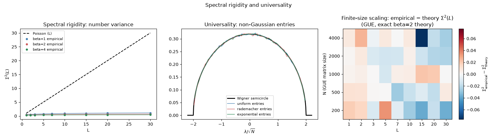
Saved rigidity_universality_replication.png

import matplotlib.pyplot as plt
import numpy as np

import physicskit.rmt as rmt

SEED = 2026

fig, axes = plt.subplots(1, 3, figsize=(16, 4.5))

# --- Panel 1: number variance rigidity ---
l_values = np.array([1, 2, 3, 5, 7, 10, 15, 20, 30])
ax = axes[0]
ax.plot(l_values, rmt.stats.number_variance_poisson(l_values), "k--", label="Poisson (L)")

for beta, cls, color in [(1, rmt.ensembles.GOE, "steelblue"), (2, rmt.ensembles.GUE, "indianred"), (4, rmt.ensembles.GSE, "seagreen")]:
    ens = cls(n=4000, seed=SEED)
    spectrum = ens.sample(n_samples=15)
    empirical = rmt.stats.number_variance_empirical(spectrum, rmt.stats.semicircle_cdf, l_values, n_windows=200, seed=SEED)
    theory = rmt.stats.number_variance_theory(l_values, beta=beta)
    ax.plot(l_values, empirical, "o", color=color, ms=4, label=f"beta={beta} empirical")
    ax.plot(l_values, theory, "-", color=color, lw=1.5, alpha=0.7)

ax.set_xlabel("L")
ax.set_ylabel(r"$\Sigma^2(L)$")
ax.set_title("Spectral rigidity: number variance")
ax.legend(fontsize=8)

# --- Panel 2: universality across entry distributions ---
ax = axes[1]
x = np.linspace(-2.2, 2.2, 400)
ax.plot(x, rmt.stats.semicircle_pdf(x), "k-", lw=2, label="Wigner semicircle")

for name, color in [
    ("uniform", "steelblue"),
    ("rademacher", "indianred"),
    ("exponential", "seagreen"),
]:
    sampler = rmt.validation.DEFAULT_ENTRY_DISTRIBUTIONS[name]
    ens = rmt.ensembles.GeneralWignerEnsemble(n=800, entry_sampler=sampler, beta=2, seed=SEED)
    spectrum = ens.sample(n_samples=20)
    centers, counts = rmt.stats.empirical_density(spectrum, bins=50)
    ax.plot(centers, counts, color=color, alpha=0.8, lw=1.3, label=f"{name} entries")

ax.set_xlabel(r"$\lambda / \sqrt{N}$")
ax.set_title("Universality: non-Gaussian entries")
ax.legend(fontsize=8)

# --- Panel 3: finite-size scaling of the number variance ---
# Panel 1 shows Sigma^2(L) at a single (large) N; here the same
# empirical estimator is stacked across MULTIPLE GUE sizes, as an
# image, to show directly how the logarithmic-rigidity theory curve is
# approached as N grows -- deviations from the beta=2 exact prediction
# shrink toward zero (lighter color) with increasing N.
n_values_fss = [200, 500, 1000, 2000, 4000]
gue_theory = rmt.stats.number_variance_theory(l_values, beta=2)

deviation_grid = np.empty((len(n_values_fss), len(l_values)))
for row, n_fss in enumerate(n_values_fss):
    ens = rmt.ensembles.GUE(n=n_fss, seed=SEED)
    spectrum = ens.sample(n_samples=10)
    empirical = rmt.stats.number_variance_empirical(spectrum, rmt.stats.semicircle_cdf, l_values, n_windows=150, seed=SEED)
    deviation_grid[row] = empirical - gue_theory

ax = axes[2]
vmax = np.abs(deviation_grid).max()
im = ax.imshow(deviation_grid, aspect="auto", origin="lower", cmap="RdBu_r", vmin=-vmax, vmax=vmax)
ax.set_xticks(range(len(l_values)))
ax.set_xticklabels([str(v) for v in l_values])
ax.set_yticks(range(len(n_values_fss)))
ax.set_yticklabels([str(v) for v in n_values_fss])
ax.set_xlabel("L")
ax.set_ylabel("N (GUE matrix size)")
ax.set_title(r"Finite-size scaling: empirical $-$ theory $\Sigma^2(L)$" + "\n(GUE, exact beta=2 theory)")
fig.colorbar(im, ax=ax, label=r"$\Sigma^2_{\rm empirical} - \Sigma^2_{\rm theory}$")

fig.suptitle("Spectral rigidity and universality")
fig.tight_layout()
out_path = "rigidity_universality_replication.png"
fig.savefig(out_path, dpi=150)
print(f"Saved {out_path}")