Kitaev’s SYK Model: Majorana Fermions, Wigner-Dyson Statistics

Unlike every classical ensemble in this package, the Sachdev-Ye-Kitaev (SYK) model is not built from i.i.d. matrix entries: it is an explicit many-body Hamiltonian acting on \(N\) Majorana fermions \(\gamma_1, \dots, \gamma_N\) (Hermitian operators satisfying the Clifford algebra \(\{\gamma_a, \gamma_b\} = 2\delta_{ab}\)),

\[H = i^{q/2} \sum_{i_1 < \cdots < i_q} J_{i_1 \cdots i_q}\, \gamma_{i_1} \cdots \gamma_{i_q},\]

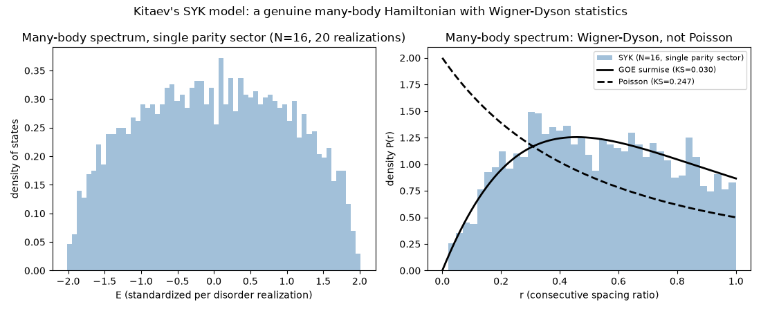
with independent random couplings \(J_{i_1\cdots i_q} \sim \mathcal{N}\!\left(0,\, \tfrac{(q-1)!\, J^2}{N^{q-1}}\right)\) for every \(q\)-index tuple (\(q=4\) here, the standard maximally chaotic case). This example builds the Sachdev-Ye-Kitaev Hamiltonian directly from physicskit.rmt.ensembles.syk.majorana_operators and verifies the Clifford algebra \(\{\gamma_a, \gamma_b\} = 2\delta_{ab}\) it must satisfy to machine precision. Then it shows the qualitative signature the SYK model is famous for: even though \(H\) is not built from i.i.d. matrix entries at all, its many-body level statistics – once restricted to a single fermion-parity sector, the two of which are otherwise uncorrelated and would wash out any repulsion signal if pooled together – are nonetheless Wigner-Dyson, not Poisson.

References: A. Kitaev, unpublished KITP talks (2015). Y.-Z. You, A. W. W. Ludwig, C. Xu, Phys. Rev. B 95 (2017) 115150 – the N mod 8 symmetry-class periodicity (N=16 here falls in the GOE class).

Run:

python examples/paper_replications/syk_demo.py

Clifford algebra {gamma_a, gamma_b} = 2*delta_ab verified for N=8: max deviation 0.00e+00 (machine precision)
Saved syk_replication.png

import matplotlib.pyplot as plt
import numpy as np
from scipy.stats import kstest

import physicskit.rmt as rmt
from physicskit.rmt.ensembles.syk import _sample_syk_hamiltonian, majorana_operators

SEED = 2026

# --- The Clifford algebra, verified directly (not plotted: the deviation
# is machine precision everywhere, so a heatmap of it is just one flat
# color and shows nothing) ---
N_CLIFFORD = 8
gammas = majorana_operators(N_CLIFFORD)
anticommutator_error = 0.0
for a in range(N_CLIFFORD):
    for b in range(N_CLIFFORD):
        target = 2.0 * np.eye(gammas[0].shape[0]) if a == b else 0.0
        anticommutator_error = max(
            anticommutator_error,
            np.abs(gammas[a] @ gammas[b] + gammas[b] @ gammas[a] - target).max(),
        )
assert anticommutator_error < 1e-10
print(f"Clifford algebra {{gamma_a, gamma_b}} = 2*delta_ab verified for N={N_CLIFFORD}: max deviation {anticommutator_error:.2e} (machine precision)")

fig, axes = plt.subplots(1, 2, figsize=(11, 4.5))

# --- Both panels below share one set of many-body spectra: the density
# of states (panel 1) and the level-spacing ratios drawn from it
# (panel 2), each computed once per trial in a single parity sector ---
N = 16
Q = 4
N_TRIALS = 20

gammas = majorana_operators(N)
dim = gammas[0].shape[0]
# Fermion parity operator: the Hermitian product of all N Majoranas
# (same i^(N/2)-phase convention the module uses to Hermitize odd
# products of Majoranas); H (built from even q=4 products) commutes
# with it, so its +1 eigenspace is an invariant, physically meaningful
# sector -- pooling both parity sectors instead would superpose two
# mutually uncorrelated spectra and wash out level repulsion.
parity = np.eye(dim, dtype=complex)
for gamma in gammas:
    parity = parity @ gamma
parity = parity * (1j ** (N // 2))
parity_eigvals, parity_eigvecs = np.linalg.eigh(parity)
sector = parity_eigvecs[:, np.round(parity_eigvals.real) == 1]

rng = np.random.default_rng(SEED)
ratios = []
pooled_eigs = []
for _ in range(N_TRIALS):
    h = _sample_syk_hamiltonian(N, Q, 1.0, rng, gammas)
    h_sector = sector.conj().T @ h @ sector
    h_sector = (h_sector + h_sector.conj().T) / 2.0
    eigs = np.linalg.eigvalsh(h_sector)
    spacings = np.diff(eigs)
    ratios.append(np.minimum(spacings[:-1], spacings[1:]) / np.maximum(spacings[:-1], spacings[1:]))
    # Standardize each disorder realization (zero mean, unit std) before
    # pooling, so trial-to-trial fluctuations in overall spectral shift
    # and width don't smear out the pooled density of states.
    pooled_eigs.append((eigs - eigs.mean()) / eigs.std())
ratios = np.concatenate(ratios)
pooled_eigs = np.concatenate(pooled_eigs)

goe_surmise = rmt.stats.RatioSurmise(beta=1)

ax = axes[0]
ax.hist(pooled_eigs, bins=60, density=True, color="steelblue", alpha=0.5)
ax.set_xlabel("E (standardized per disorder realization)")
ax.set_ylabel("density of states")
ax.set_title(f"Many-body spectrum, single parity sector (N={N}, {N_TRIALS} realizations)")


def poisson_ratio_cdf(r: np.ndarray) -> np.ndarray:
    return 2.0 * r / (1.0 + r)


ks_goe = kstest(ratios, goe_surmise.cdf).statistic
ks_poisson = kstest(ratios, poisson_ratio_cdf).statistic

r_grid = np.linspace(0, 1, 400)
ax = axes[1]
ax.hist(ratios, bins=40, density=True, alpha=0.5, color="steelblue", label=f"SYK (N={N}, single parity sector)")
ax.plot(r_grid, goe_surmise.pdf(r_grid), "k-", lw=2, label=f"GOE surmise (KS={ks_goe:.3f})")
ax.plot(r_grid, 2.0 / (1.0 + r_grid) ** 2, "k--", lw=2, label=f"Poisson (KS={ks_poisson:.3f})")
ax.set_xlabel("r (consecutive spacing ratio)")
ax.set_ylabel("density P(r)")
ax.set_title("Many-body spectrum: Wigner-Dyson, not Poisson")
ax.legend(fontsize=8)

fig.suptitle(
    "Kitaev's SYK model: a genuine many-body Hamiltonian with Wigner-Dyson statistics",
)
fig.tight_layout()
out_path = "syk_replication.png"
fig.savefig(out_path, dpi=150)
print(f"Saved {out_path}")