Tracy-Widom Soft-Edge Laws

For the Gaussian beta-ensembles GOE (\(\beta=1\)), GUE (\(\beta=2\)), and GSE (\(\beta=4\)), the bulk of the \(n\)-eigenvalue spectrum fills the semicircle \([-2, 2]\), but the largest eigenvalue \(\lambda_{\max}\) fluctuates above the edge \(2\) on a much finer scale than the bulk spacing: rescaling

\[s = n^{2/3}(\lambda_{\max} - 2) \;\;(\beta=1,2), \qquad s = (2n)^{2/3}(\lambda_{\max} - 2) \;\;(\beta=4)\]

converges in distribution to the Tracy-Widom law \(F_\beta(s)\), the universal “soft edge” statistic shared by a wide class of random matrix and growth-process models.

All three laws are built from \(q(x)\), the Hastings-McLeod solution of the Painleve II equation \(q''(x) = x q(x) + 2 q(x)^3\) with \(q(x) \sim \mathrm{Ai}(x)\) as \(x \to +\infty\), via

\[F_2(s) = \exp\left(-\int_s^\infty (x-s)\, q(x)^2\, dx\right),\]

\[F_1(s) = \sqrt{F_2(s)}\, \exp\left(-\tfrac{1}{2}\int_s^\infty q(x)\, dx\right), \qquad F_4(s) = \sqrt{F_2(s)}\, \cosh\left(\tfrac{1}{2}\int_s^\infty q(x)\, dx\right).\]

This example draws \(\lambda_{\max}\) from Monte Carlo GOE/GUE/GSE samples, rescales it as above, and overlays the resulting histogram against the corresponding \(F_1\), \(F_2\), or \(F_4\) density obtained by numerically integrating the Painleve II equation.

References: C. A. Tracy, H. Widom, Commun. Math. Phys. 159 (1994) 151. C. A. Tracy, H. Widom, Commun. Math. Phys. 177 (1996) 727.

Run:

python examples/paper_replications/tracy_widom_demo.py

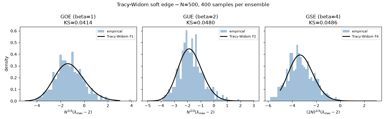
Saved tracy_widom_replication.png

import matplotlib.pyplot as plt
import numpy as np

import physicskit.rmt as rmt

N = 500
N_SAMPLES = 400
SEED = 2026

fig, axes = plt.subplots(1, 3, figsize=(13, 4), sharey=True)
s_grid = np.linspace(-5, 3, 400)

for ax, (label, cls, beta) in zip(
    axes,
    [("GOE (beta=1)", rmt.ensembles.GOE, 1), ("GUE (beta=2)", rmt.ensembles.GUE, 2), ("GSE (beta=4)", rmt.ensembles.GSE, 4)],
    strict=True,
):
    ensemble = cls(n=N, seed=SEED)
    spectrum = ensemble.sample(n_samples=N_SAMPLES)
    benchmark = rmt.validation.TracyWidom(beta=beta)
    result = benchmark.validate(spectrum, seed=SEED)

    lam_max = rmt.stats.largest_eigenvalues(spectrum)
    scale = rmt.stats.tracy_widom_edge_scale(N, beta)
    edge_stat = scale * (lam_max - 2.0)

    ax.hist(edge_stat, bins=40, density=True, alpha=0.5, color="steelblue", label="empirical")
    theory_cdf = rmt.stats.tracy_widom_cdf(s_grid, beta)
    theory_pdf = np.gradient(theory_cdf, s_grid)
    tw_index = {1: 1, 2: 2, 4: 4}[beta]
    ax.plot(s_grid, theory_pdf, "k-", lw=2, label=f"Tracy-Widom F{tw_index}")
    ax.set_title(f"{label}\nKS={result.ks_statistic:.4f}")
    xlabel = r"$N^{2/3}(\lambda_{max} - 2)$" if beta != 4 else r"$(2N)^{2/3}(\lambda_{max} - 2)$"
    ax.set_xlabel(xlabel)
    ax.legend(fontsize=8)

axes[0].set_ylabel("density")
fig.suptitle(f"Tracy-Widom soft edge -- N={N}, {N_SAMPLES} samples per ensemble")
fig.tight_layout()
out_path = "tracy_widom_replication.png"
fig.savefig(out_path, dpi=150)
print(f"Saved {out_path}")