Wishart’s Sample Covariance Matrix

For an \(m \times n\) data matrix \(X\) of \(m\) independent samples of \(n\) variables, the sample covariance (scatter) matrix

\[S = \frac{X^T X}{m}\]

has, for \(X\) with real, complex, or quaternionic i.i.d. Gaussian entries, eigenvalues that are exactly those of physicskit’s LOE (\(\beta=1\)), LUE (\(\beta=2\)), and LSE (\(\beta=4\)) ensembles respectively – not merely asymptotically, but for any finite \(n\) and \(m\). As \(m \to \infty\) at fixed aspect ratio \(\gamma = n/m\), the eigenvalues of \(S\) converge to the Marchenko-Pastur law on \([(1-\sqrt{\gamma})^2, (1+\sqrt{\gamma})^2]\).

This example reproduces Wishart’s original (1928) construction directly: for an m x n data matrix X of independent samples, the sample covariance (scatter) matrix S = X^T X / m has eigenvalues that are exactly those of physicskit’s LOE/LUE/LSE ensembles, for real, complex, and quaternion entries respectively – not merely asymptotically, but for any finite n and m. This is the statistical-multivariate-analysis construction that predates Wigner’s use of random matrices in physics by three decades.

Reference: J. Wishart, Biometrika 20A (1928) 32.

Run:

python examples/paper_replications/wishart_demo.py

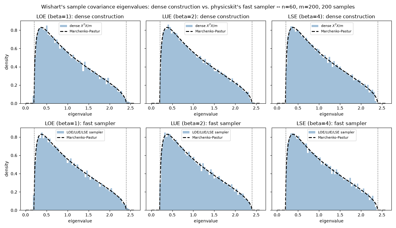
Saved wishart_replication.png

import matplotlib.pyplot as plt
import numpy as np

import physicskit.rmt as rmt

N = 60
M = 200
N_SAMPLES = 200
SEED = 2026

rng = np.random.default_rng(SEED)
gamma = N / M
lo, hi = rmt.stats.mp_support(gamma)
x_grid = np.linspace(max(lo - 0.2, 0), hi + 0.2, 400)

fig, axes = plt.subplots(2, 3, figsize=(13, 7.5), sharey=True)


def dense_wishart_eigs(rng: np.random.Generator, n: int, m: int, beta: int) -> np.ndarray:
    """Eigenvalues of S = X^T X / m for an explicit m x n data matrix X,
    built entry-by-entry (not via the tridiagonal fast sampler)."""
    if beta == 1:
        x = rng.standard_normal((m, n))
        s = x.T @ x / m
        return np.linalg.eigvalsh(s)
    if beta == 2:
        x = (rng.standard_normal((m, n)) + 1j * rng.standard_normal((m, n))) / np.sqrt(2.0)
        s = x.conj().T @ x / m
        return np.linalg.eigvalsh(s)
    # beta == 4: quaternion data matrix, embedded as a 2m x 2n complex
    # matrix via the same quaternion-to-2x2-complex-block map used by
    # physicskit.rmt.ensembles.GinSE.
    a = rng.standard_normal((m, n))
    b = rng.standard_normal((m, n))
    c = rng.standard_normal((m, n))
    d = rng.standard_normal((m, n))
    xq = np.zeros((2 * m, 2 * n), dtype=complex)
    xq[0::2, 0::2] = (a + 1j * b) / 2.0
    xq[0::2, 1::2] = (c + 1j * d) / 2.0
    xq[1::2, 0::2] = (-c + 1j * d) / 2.0
    xq[1::2, 1::2] = (a - 1j * b) / 2.0
    s = xq.conj().T @ xq / m
    eigs = np.linalg.eigvalsh(s)
    return eigs[0::2]  # exact Kramers double degeneracy -- keep one per pair


for col, (label, cls, beta) in enumerate(
    [("LOE (beta=1)", rmt.ensembles.LOE, 1), ("LUE (beta=2)", rmt.ensembles.LUE, 2), ("LSE (beta=4)", rmt.ensembles.LSE, 4)]
):
    dense_eigs = np.concatenate([dense_wishart_eigs(rng, N, M, beta) for _ in range(N_SAMPLES)])

    ensemble = cls(n=N, m=M, seed=SEED + col + 1)
    fast_eigs = ensemble.sample(n_samples=N_SAMPLES).eigenvalues.ravel()

    ax = axes[0, col]
    ax.hist(dense_eigs, bins=60, density=True, alpha=0.5, color="steelblue", label=r"dense $X^T X / m$")
    ax.plot(x_grid, rmt.stats.mp_pdf(x_grid, gamma), "k--", lw=2, label="Marchenko-Pastur")
    ax.axvline(lo, color="gray", ls="--", lw=1)
    ax.axvline(hi, color="gray", ls="--", lw=1)
    ax.set_title(f"{label}: dense construction")
    ax.set_xlabel("eigenvalue")
    ax.legend(fontsize=8)

    ax = axes[1, col]
    ax.hist(fast_eigs, bins=60, density=True, alpha=0.5, color="steelblue", label="LOE/LUE/LSE sampler")
    ax.plot(x_grid, rmt.stats.mp_pdf(x_grid, gamma), "k--", lw=2, label="Marchenko-Pastur")
    ax.axvline(lo, color="gray", ls="--", lw=1)
    ax.axvline(hi, color="gray", ls="--", lw=1)
    ax.set_title(f"{label}: fast sampler")
    ax.set_xlabel("eigenvalue")
    ax.legend(fontsize=8)

axes[0, 0].set_ylabel("density")
axes[1, 0].set_ylabel("density")
fig.suptitle(
    f"Wishart's sample covariance eigenvalues: dense construction vs. physicskit's fast sampler -- n={N}, m={M}, {N_SAMPLES} samples",
)
fig.tight_layout()
out_path = "wishart_replication.png"
fig.savefig(out_path, dpi=150)
print(f"Saved {out_path}")