The Ehrenfest time: the log(1/ħ) breakdown of correspondence

Ehrenfest’s theorem says a narrow wavepacket’s centre obeys Newton’s equations as long as the packet stays small compared with the scale on which the force varies. Berman and Zaslavsky (1978) asked how long that lasts when the classical motion is chaotic. A minimum-uncertainty packet starts with width of order \(\sqrt\hbar\), and chaos stretches it by \(e^{\lambda t}\), with \(\lambda\) the Lyapunov exponent. The packet reaches the size of the system, and stops following any single trajectory, after

\[t_E \simeq \frac{1}{2\lambda}\ln\frac{1}{\hbar} + \text{const}.\]

This time grows only logarithmically as \(\hbar\to0\): halving \(\hbar\) buys a fixed number of extra steps. In an integrable system the packet spreads only as a power of \(t\), and correspondence lasts for a time that grows as a power of \(1/\hbar\).

This example measures \(t_E\) in the kicked rotor, the quantized standard map \(p'=p+K\sin\theta,\ \theta'=\theta+p'\) on the torus (QuantumKickedRotor), with \(\hbar=2\pi/N\) set by the Hilbert-space dimension \(N\).

import matplotlib.pyplot as plt
import numpy as np

from physicskit.chaos.quantum.maps import QuantumKickedRotor
from physicskit.chaos.systems.maps import StandardMap

K = 6.0  # strongly chaotic
classical = StandardMap(k=K)

The Lyapunov exponent

Iterate the tangent map \(J=\begin{pmatrix}1+K\cos\theta & 1\\ K\cos\theta & 1\end{pmatrix}\) along a long orbit. For large \(K\) the result is close to \(\ln(K/2)\).

orbit = classical.trajectory(np.array([1.0, 2.0]), n_iter=50_000)
v, log_growth = np.array([1.0, 0.0]), 0.0
for theta in orbit[:-1, 0]:
    c = K * np.cos(theta)
    v = np.array([(1 + c) * v[0] + v[1], c * v[0] + v[1]])
    norm = np.linalg.norm(v)
    log_growth += np.log(norm)
    v /= norm
lam = log_growth / (len(orbit) - 1)
print(f"Lyapunov exponent lambda = {lam:.3f}  (ln(K/2) = {np.log(K / 2):.3f})")

Lyapunov exponent lambda = 1.135  (ln(K/2) = 1.099)

A packet leaves its trajectory

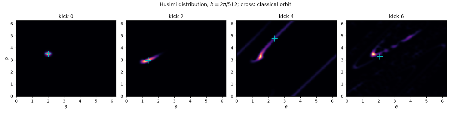
Follow a coherent state and the classical orbit from its centre. The Husimi distribution stays a compact blob around the classical point for a few kicks, then is stretched along the unstable direction and folded over the torus.

dim = 512
rotor = QuantumKickedRotor(k=K, dim=dim)
theta0, p0 = 2.0, 3.5
states = rotor.evolve(rotor.coherent_state(theta0, p0), n_steps=6)
traj = classical.trajectory(np.array([theta0, p0]), n_iter=6)

fig1, axes = plt.subplots(1, 4, figsize=(15, 3.8))
for ax, n in zip(axes, (0, 2, 4, 6)):
    Th, P, H = rotor.husimi(states[n], resolution=120)
    ax.pcolormesh(Th, P, H, cmap="magma", shading="auto")
    ax.plot(*traj[n], "c+", ms=14, mew=2)
    ax.set_title(f"kick {n}")
    ax.set_xlabel(r"$\theta$")
axes[0].set_ylabel("p")
fig1.suptitle(rf"Husimi distribution, $\hbar = 2\pi/{dim}$; cross: classical orbit")
fig1.tight_layout()

Measuring the Ehrenfest time

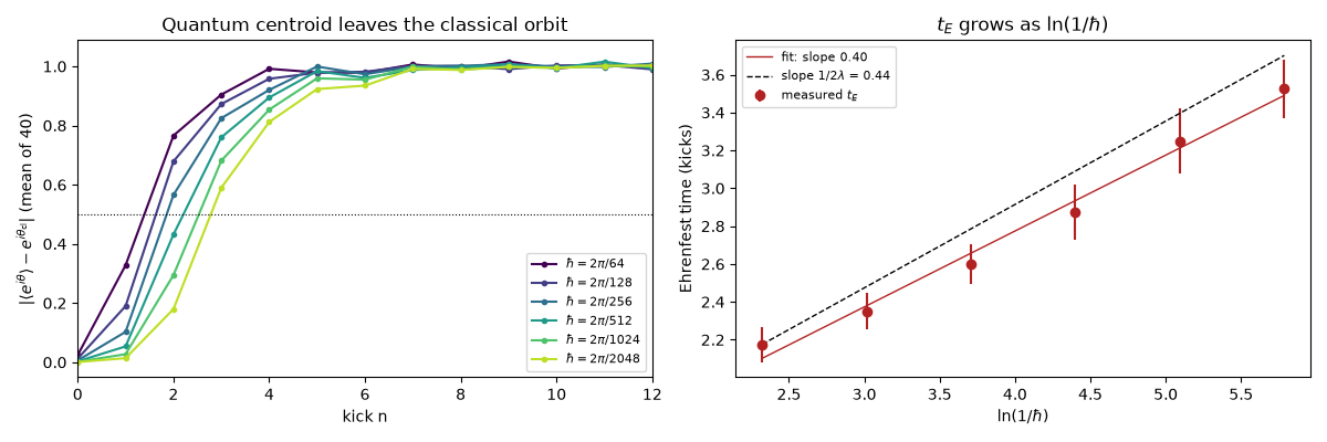
Take the quantum mean of \(e^{i\theta}\); while the packet is narrow it sits on the unit circle at the classical angle. Define \(t_E\) as the first kick at which it is more than 0.5 away from \(e^{i\theta_{\rm cl}}\), and average over 40 random starting points, since the local stretching rate fluctuates along an orbit.

rng = np.random.default_rng(1)
centres = rng.uniform(0, 2 * np.pi, size=(40, 2))
dims = [64, 128, 256, 512, 1024, 2048]
n_kicks = 30

fig2, (ax1, ax2) = plt.subplots(1, 2, figsize=(12, 4))
t_E, t_E_err, hbars = [], [], []
for dim, color in zip(dims, plt.cm.viridis(np.linspace(0, 0.9, len(dims)))):
    rotor = QuantumKickedRotor(k=K, dim=dim)
    U = rotor.floquet_operator()
    theta = 2 * np.pi * np.arange(dim) / dim
    deviations, crossings = [], []
    for th0, pp0 in centres:
        psi = rotor.coherent_state(th0, pp0)
        orbit = classical.trajectory(np.array([th0, pp0]), n_iter=n_kicks)
        dev = np.empty(n_kicks + 1)
        for n in range(n_kicks + 1):
            dev[n] = abs(np.sum(np.abs(psi) ** 2 * np.exp(1j * theta)) - np.exp(1j * orbit[n, 0]))
            psi = U @ psi
        deviations.append(dev)
        crossings.append(np.argmax(dev > 0.5))
    hbars.append(rotor.hbar)
    t_E.append(np.mean(crossings))
    t_E_err.append(np.std(crossings) / np.sqrt(len(crossings)))
    ax1.plot(np.arange(n_kicks + 1), np.mean(deviations, axis=0), "o-", ms=3, color=color, label=rf"$\hbar=2\pi/{dim}$")
ax1.axhline(0.5, color="k", ls=":", lw=0.8)
ax1.set_xlim(0, 12)
ax1.set_xlabel("kick n")
ax1.set_ylabel(r"$|\langle e^{i\theta}\rangle - e^{i\theta_{\rm cl}}|$ (mean of 40)")
ax1.set_title("Quantum centroid leaves the classical orbit")
ax1.legend(fontsize=8)

log_inv_hbar = np.log(1 / np.array(hbars))
slope, intercept = np.polyfit(log_inv_hbar, t_E, 1)
ax2.errorbar(log_inv_hbar, t_E, yerr=t_E_err, fmt="o", color="firebrick", label=r"measured $t_E$")
ax2.plot(log_inv_hbar, intercept + slope * log_inv_hbar, color="firebrick", lw=1, label=f"fit: slope {slope:.2f}")
ax2.plot(log_inv_hbar, t_E[0] + (log_inv_hbar - log_inv_hbar[0]) / (2 * lam), "k--", lw=1, label=rf"slope $1/2\lambda$ = {1 / (2 * lam):.2f}")
ax2.set_xlabel(r"$\ln(1/\hbar)$")
ax2.set_ylabel("Ehrenfest time (kicks)")
ax2.set_title(r"$t_E$ grows as $\ln(1/\hbar)$")
ax2.legend(fontsize=8)
fig2.tight_layout()

for d, hb, t in zip(dims, hbars, t_E):
    print(f"N = {d:5d}, hbar = {hb:.5f}: t_E = {t:.2f} kicks")
print(f"fitted slope dt_E / dln(1/hbar) = {slope:.3f}; prediction 1/(2 lambda) = {1 / (2 * lam):.3f}")

plt.show()

N =    64, hbar = 0.09817: t_E = 2.17 kicks
N =   128, hbar = 0.04909: t_E = 2.35 kicks
N =   256, hbar = 0.02454: t_E = 2.60 kicks
N =   512, hbar = 0.01227: t_E = 2.88 kicks
N =  1024, hbar = 0.00614: t_E = 3.25 kicks
N =  2048, hbar = 0.00307: t_E = 3.52 kicks
fitted slope dt_E / dln(1/hbar) = 0.401; prediction 1/(2 lambda) = 0.440

Check

For K = 6 the standard map’s Lyapunov exponent is close to ln(K/2), and the Ehrenfest time grows as ln(1/hbar) / 2 lambda.

assert abs(lam - np.log(K / 2)) < 0.1
assert np.all(np.diff(t_E) > 0)
assert abs(slope * 2 * lam - 1) < 0.2