Feynman paths and the classical limit

Feynman’s path-integral formulation (Feynman & Hibbs 1965, building on Dirac’s 1933 “The Lagrangian in Quantum Mechanics”) writes the quantum propagator as a sum over every continuous path \(x(t)\) connecting fixed endpoints, each weighted by a phase built from its classical action \(S[x(t)]\). The same construction also applies to the harmonic oscillator, whose classical path curves rather than running straight between the fixed endpoints (harmonic_oscillator_classical_path(), harmonic_oscillator_classical_action()), showing that the same closest-to-classical-first phasor concentration at small \(\hbar\) is not an artifact of the free particle’s trivially straight classical trajectory:

\[K(x_f,T;x_0,0) = \int \mathcal{D}[x(t)]\; \exp\!\left(\frac{i}{\hbar}S[x(t)]\right).\]

Near the true classical (stationary-action) trajectory, \(S\) barely changes from one nearby path to the next, so their phasors stay aligned and reinforce; far away, \(S\) varies rapidly and the phasors spin through many turns, largely cancelling. Shrinking \(\hbar\) makes the phase \(S/\hbar\) more sensitive to path deformations, shrinking the “aligned” neighborhood of the classical path – in the limit \(\hbar\to 0\) only the classical path survives, recovering the principle of stationary action. This is demonstrated below for the free particle, whose classical path and action are known in closed form (free_particle_classical_path(), free_particle_classical_action()), so every result here can be checked exactly, then repeated for the harmonic oscillator’s curved classical path.

import matplotlib.pyplot as plt
import numpy as np

from physicskit.semiclassical.core.path_integral import build_phasor_diagram
from physicskit.semiclassical.visualizers.path_integral import animate_feynman_phasor_spiral, plot_phasor_convergence

x0, xf, T, m = 0.0, 1.0, 1.0, 1.0
n_slices, n_paths, sigma, seed = 40, 400, 0.5, 42

hbar_large, hbar_small = 20.0, 1.0

data_large = build_phasor_diagram(x0, xf, T, m, hbar_large, potential="free", n_slices=n_slices, n_paths=n_paths, sigma=sigma, seed=seed)
data_small = build_phasor_diagram(x0, xf, T, m, hbar_small, potential="free", n_slices=n_slices, n_paths=n_paths, sigma=sigma, seed=seed)

paths, actions, x_cl, S_cl, partial_large = data_large
_, _, _, _, partial_small = data_small
t = np.linspace(0.0, T, x_cl.shape[0])

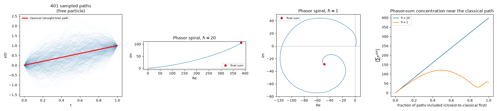
Sampled paths, and the growing Feynman phasor sum at two very different values of hbar ————————————————————————– Both phasor panels use the same ensemble of sampled paths, added in the same closest-to-classical-first order – only hbar differs. At the large hbar the phasors barely notice which path they came from and the sum wanders like a random walk from the very first steps; at the small hbar the phasors near the classical path stay tightly aligned before the more distant paths start spinning around and stall the sum’s growth.

order = np.argsort(np.abs(actions - S_cl))

fig, axes = plt.subplots(1, 4, figsize=(20, 4.5))

axes[0].plot(t, paths[order].T, color="C0", alpha=0.05, lw=0.8)
axes[0].plot(t, x_cl, color="red", lw=2.5, label="classical (straight-line) path")
axes[0].set_xlabel("t")
axes[0].set_ylabel("x(t)")
axes[0].set_title(f"{paths.shape[0]} sampled paths\n(free particle)")
axes[0].legend(fontsize=8)

for ax, partial, hbar in [(axes[1], partial_large, hbar_large), (axes[2], partial_small, hbar_small)]:
    ax.plot(partial.real, partial.imag, color="C0", lw=1.0)
    ax.plot(partial[-1].real, partial[-1].imag, "o", color="crimson", label="final sum")
    ax.axhline(0, color="gray", lw=0.5)
    ax.axvline(0, color="gray", lw=0.5)
    ax.set_aspect("equal")
    ax.set_xlabel("Re")
    ax.set_ylabel("Im")
    ax.set_title(rf"Phasor spiral, $\hbar={hbar:g}$")
    ax.legend(fontsize=8)

plot_phasor_convergence([partial_large, partial_small], [hbar_large, hbar_small], ax=axes[3])

fig.tight_layout()

Sanity checks

n_total = partial_large.shape[0] - 1
idx_10pct = max(1, round(0.1 * n_total))
frac_large = abs(partial_large[idx_10pct]) / abs(partial_large[-1])
frac_small = abs(partial_small[idx_10pct]) / abs(partial_small[-1])

print(f"Classical straight-line action S_cl = {S_cl:.6f}")
print(f"Number of sampled paths (incl. classical): {paths.shape[0]}")
print("Fraction of final phasor magnitude from closest 10% of paths:")
print(f"  hbar = {hbar_large:g} (large): {frac_large:.4f}")
print(f"  hbar = {hbar_small:g} (small): {frac_small:.4f}")
print(f"Concentration increases as hbar shrinks: {frac_small > frac_large}")

Classical straight-line action S_cl = 0.500000
Number of sampled paths (incl. classical): 401
Fraction of final phasor magnitude from closest 10% of paths:
  hbar = 20 (large): 0.1005
  hbar = 1 (small): 0.6358
Concentration increases as hbar shrinks: True

The same construction for a curved classical path: the harmonic oscillator ————————————————————————– Repeating the whole phasor-diagram construction with potential="harmonic" swaps in the harmonic oscillator’s curved classical trajectory (harmonic_oscillator_classical_path()) in place of the free particle’s straight line, showing that the same stationary-action concentration mechanism – and the same growing concentration as \(\hbar\) shrinks – holds regardless of the classical path’s shape.

omega = 2.5
data_h_large = build_phasor_diagram(x0, xf, T, m, hbar_large, potential="harmonic", omega=omega, n_slices=n_slices, n_paths=n_paths, sigma=sigma, seed=seed)
data_h_small = build_phasor_diagram(x0, xf, T, m, hbar_small, potential="harmonic", omega=omega, n_slices=n_slices, n_paths=n_paths, sigma=sigma, seed=seed)

paths_h, actions_h, x_cl_h, S_cl_h, partial_h_large = data_h_large
_, _, _, _, partial_h_small = data_h_small
order_h = np.argsort(np.abs(actions_h - S_cl_h))

fig_h, axes_h = plt.subplots(1, 3, figsize=(15, 4.5))

axes_h[0].plot(t, paths_h[order_h].T, color="C0", alpha=0.05, lw=0.8)
axes_h[0].plot(t, x_cl_h, color="red", lw=2.5, label="classical path (harmonic)")
axes_h[0].set_xlabel("t")
axes_h[0].set_ylabel("x(t)")
axes_h[0].set_title(f"{paths_h.shape[0]} sampled paths\n(harmonic oscillator, omega={omega:g})")
axes_h[0].legend(fontsize=8)

for ax, partial, hbar in [(axes_h[1], partial_h_large, hbar_large), (axes_h[2], partial_h_small, hbar_small)]:
    ax.plot(partial.real, partial.imag, color="C0", lw=1.0)
    ax.plot(partial[-1].real, partial[-1].imag, "o", color="crimson", label="final sum")
    ax.axhline(0, color="gray", lw=0.5)
    ax.axvline(0, color="gray", lw=0.5)
    ax.set_aspect("equal")
    ax.set_xlabel("Re")
    ax.set_ylabel("Im")
    ax.set_title(rf"Phasor spiral (harmonic), $\hbar={hbar:g}$")
    ax.legend(fontsize=8)

fig_h.tight_layout()

frac_h_large = abs(partial_h_large[idx_10pct]) / abs(partial_h_large[-1])
frac_h_small = abs(partial_h_small[idx_10pct]) / abs(partial_h_small[-1])
print(f"Harmonic oscillator classical action S_cl = {S_cl_h:.6f}")
print("Fraction of final phasor magnitude from closest 10% of paths (harmonic):")
print(f"  hbar = {hbar_large:g} (large): {frac_h_large:.4f}")
print(f"  hbar = {hbar_small:g} (small): {frac_h_small:.4f}")
print(f"Concentration increases as hbar shrinks (harmonic): {frac_h_small > frac_h_large}")

plt.show()

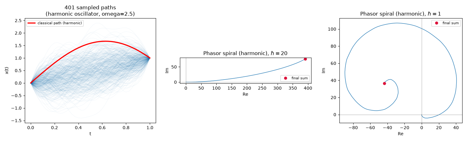
Harmonic oscillator classical action S_cl = -1.673310
Fraction of final phasor magnitude from closest 10% of paths (harmonic):
  hbar = 20 (large): 0.1005
  hbar = 1 (small): 0.6107
Concentration increases as hbar shrinks (harmonic): True

Animation: paths joining the phasor sum one at a time

The static spiral above already shows the endpoint; watching it build up path by path – closest to the classical trajectory first – makes the reinforce-then-cancel mechanism directly visible: the arrow chain marches steadily in one direction while only the near-classical paths are being added, then starts curling into tight, self-cancelling loops once the more distant, rapidly-varying-action paths join in.

anim = animate_feynman_phasor_spiral(paths, actions, x_cl, S_cl, hbar_small, t, interval=40)
plt.show()

To save the animation to a file instead of (or in addition to) displaying it interactively, use e.g.:

anim.save("feynman_phasor_spiral.gif", writer="pillow", fps=20)