Heller’s time-dependent spectroscopy: absorption bands from short-time dynamics

Heller (1981) recast molecular absorption spectroscopy in the time domain. A photon lifts the vibrational ground state \(\psi_0\) of the lower electronic surface onto the upper surface, where it is no longer stationary. The absorption spectrum is the Fourier transform of the autocorrelation of the packet that then moves on the upper surface,

\[\sigma(E) \propto \int_{-\infty}^{\infty}\langle\psi_0|\psi(t)\rangle\, e^{iEt/\hbar}\,dt = 2\pi\hbar\sum_n|\langle n|\psi_0\rangle|^2\,\delta(E-E_n),\]

the Franck-Condon factors of the upper surface’s levels. The time-domain view explains the spectrum by events of the packet’s motion. Its departure from the Franck-Condon region, within a fraction of a period, sets the width of the whole band. Its return after a vibrational period, if the upper surface is bound, splits the band into a progression. The individual lines need the long-time signal. The first two stages take a period or two, so short-time semiclassical dynamics already accounts for the band shape and the progression.

This example uses one thawed Gaussian (thawed_gaussian_propagate()) on two upper surfaces, a bound Morse curve and a repulsive one, and compares the spectra with the exact Franck-Condon factors (NumerovSolver) and with split-operator evolution (SplitOperatorSolver1D). Units: \(\hbar=m=1\).

import matplotlib.pyplot as plt
import numpy as np
from numba import njit

from physicskit.quantum.core.eigensolvers import NumerovSolver
from physicskit.quantum.core.solvers import SplitOperatorSolver1D
from physicskit.semiclassical.core.propagators import frozen_gaussian_1d, thawed_gaussian_propagate, thawed_gaussian_wavefunction

# Ground surface: harmonic, omega = 2, so the initial packet is a Gaussian
# with gamma = omega / 2 = 1 centred at x = 0.
gamma0 = 1.0
x = np.linspace(-8, 88, 8192)
dx = x[1] - x[0]
psi0 = frozen_gaussian_1d(x, 0.0, 0.0, gamma0)

# Bound upper surface: Morse well displaced to x = d, raised by T_e.
D_e, a_m, d, T_e = 40.0, 0.25, 2.0, 10.0
morse_params = np.array([D_e, a_m, d, T_e])


@njit
def V_morse(q, params):
    return params[3] + params[0] * (1 - np.exp(-params[1] * (q - params[2]))) ** 2


@njit
def dV_morse(q, params):
    e = np.exp(-params[1] * (q - params[2]))
    return 2 * params[0] * params[1] * e * (1 - e)


@njit
def d2V_morse(q, params):
    e = np.exp(-params[1] * (q - params[2]))
    return 2 * params[0] * params[1] ** 2 * e * (2 * e - 1)


# Repulsive upper surface: an exponential wall.
A_r, b_r = 16.0, 0.6
rep_params = np.array([A_r, b_r])


@njit
def V_rep(q, params):
    return params[0] * np.exp(-params[1] * q)


@njit
def dV_rep(q, params):
    return -params[0] * params[1] * np.exp(-params[1] * q)


@njit
def d2V_rep(q, params):
    return params[0] * params[1] ** 2 * np.exp(-params[1] * q)


omega_e = a_m * np.sqrt(2 * D_e)
T_vib = 2 * np.pi / omega_e
dt = 0.004
n_steps = int(round(6 * T_vib / dt))
save = 5


def autocorrelations(V, dV, d2V, params):
    _, q, p, alpha, s = thawed_gaussian_propagate(0.0, 0.0, gamma0, dV, d2V, V, 1.0, dt, n_steps, params=params)
    ks = np.arange(0, n_steps + 1, save)
    C_tg = np.array([np.sum(psi0.conj() * thawed_gaussian_wavefunction(x, q[k], p[k], alpha[k], s[k])) * dx for k in ks])
    solver = SplitOperatorSolver1D(x, lambda xx: V(xx, params), dt=dt)
    frames, times = solver.propagate(psi0, n_steps, save_every=save)
    C_ex = np.array([np.sum(psi0.conj() * f) * dx for f in frames])
    return times, C_ex, C_tg


def spectrum(E, times, C, t_window):
    w = np.exp(-0.5 * (times / t_window) ** 2)
    dts = times[1] - times[0]
    return (2 * np.real(np.exp(1j * np.outer(E, times)) @ (C * w)) - (C[0] * w[0]).real) * dts / (2 * np.pi)


times, C_morse_ex, C_morse_tg = autocorrelations(V_morse, dV_morse, d2V_morse, morse_params)
_, C_rep_ex, C_rep_tg = autocorrelations(V_rep, dV_rep, d2V_rep, rep_params)

The two upper surfaces

The vertical transition puts the packet on the steep inner side of the displaced Morse curve, or on the repulsive wall. Either way it starts to slide downhill at once.

fig1, (ax1, ax2) = plt.subplots(1, 2, figsize=(12, 4))
xx = np.linspace(-2.5, 9, 400)
ax1.plot(xx, 2 * xx**2, color="0.5", label="ground surface")
ax1.plot(xx, [V_morse(v, morse_params) for v in xx], color="steelblue", label="bound upper surface (Morse)")
ax1.plot(xx, [V_rep(v, rep_params) for v in xx], color="firebrick", label="repulsive upper surface")
ax1.fill_between(xx, 1.0, 1.0 + 3 * np.abs(frozen_gaussian_1d(xx, 0, 0, gamma0)) ** 2, color="0.5", alpha=0.4)
ax1.annotate("", (0, V_morse(0.0, morse_params)), (0, 1.1), arrowprops=dict(arrowstyle="->", color="k"))
ax1.set_ylim(0, 30)
ax1.set_xlabel("vibrational coordinate x")
ax1.set_ylabel("energy")
ax1.set_title("Vertical (Franck-Condon) excitation")
ax1.legend(fontsize=8)

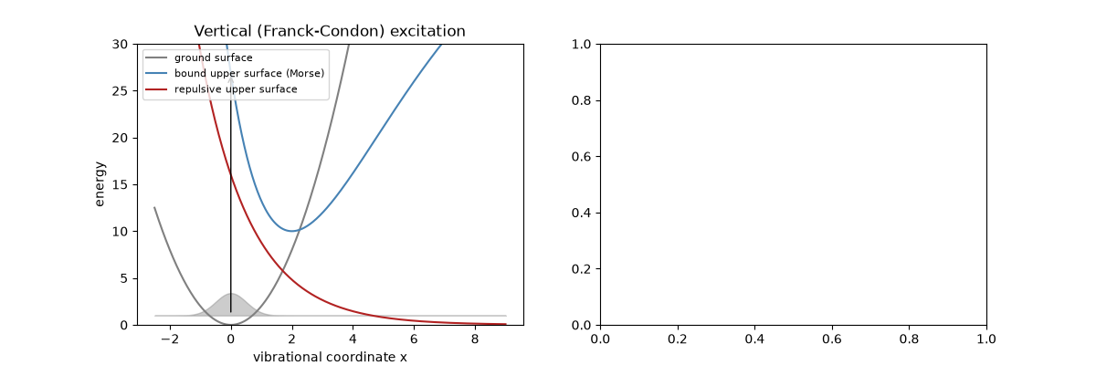
<matplotlib.legend.Legend object at 0x3728e5880>

Autocorrelation: departure and return

On both surfaces \(|C(t)|\) first falls as the packet leaves, and the thawed Gaussian follows that decay closely. On the Morse surface the packet comes back a little more than one small-oscillation period later (the well softens with energy). The thawed Gaussian comes back at about the right time, but as a single, strongly stretched Gaussian it gets the shape of the return only roughly. On the repulsive surface the packet never returns.

ax2.plot(times / T_vib, np.abs(C_morse_ex), color="steelblue", lw=3, alpha=0.4, label="Morse, exact")
ax2.plot(times / T_vib, np.abs(C_morse_tg), color="steelblue", lw=1, label="Morse, thawed Gaussian")
ax2.plot(times / T_vib, np.abs(C_rep_ex), color="firebrick", lw=3, alpha=0.4, label="repulsive, exact")
ax2.plot(times / T_vib, np.abs(C_rep_tg), color="firebrick", lw=1, label="repulsive, thawed Gaussian")
ax2.set_xlim(0, 3)
ax2.set_xlabel(r"t / $T_{\rm vib}$")
ax2.set_ylabel(r"$|\langle\psi_0|\psi(t)\rangle|$")
ax2.set_title("Autocorrelation on the upper surface")
ax2.legend(fontsize=8)
fig1.tight_layout()

Spectra

The exact Franck-Condon factors are drawn as sticks. A short time window, about a quarter period, sees only the departure and gives the smooth band. Heller’s estimate of it is a Gaussian centred at the vertical energy \(V_e(0)\) with width \(|V_e'(0)|\sigma_x\), the slope of the upper surface times the packet width. A window of about one period (\(\sigma_t=0.8\,T\)) includes the first return and splits the band into the vibrational progression, which the thawed Gaussian reproduces near the band centre and less well towards its edges. For the repulsive surface there is no return and no progression.

E = np.linspace(0, 40, 2000)
sigma_x = np.sqrt(1 / (4 * gamma0))
res = NumerovSolver(np.linspace(-4, 30, 3000), lambda r: V_morse(r, morse_params)).solve(n_states=16)
fc = np.array([np.trapezoid(w * np.exp(-gamma0 * res.x**2) * (2 * gamma0 / np.pi) ** 0.25, res.x) ** 2 for w in res.wavefunctions])

fig2, (ax3, ax4) = plt.subplots(1, 2, figsize=(12, 4))
for t_win, color in [(0.25 * T_vib, "0.5"), (0.8 * T_vib, "steelblue")]:
    ax3.plot(E, spectrum(E, times, C_morse_ex, t_win), color=color, lw=3, alpha=0.4)
    ax3.plot(E, spectrum(E, times, C_morse_tg, t_win), color=color, lw=1, ls="--", label=f"thawed, window {t_win / T_vib:.2f} T")
# A line of weight |c_n|^2 seen through a Gaussian window of length tau peaks at |c_n|^2 tau / sqrt(2 pi).
ax3.vlines(res.energies, 0, fc * 0.8 * T_vib / np.sqrt(2 * np.pi), color="k", lw=1.5, label="exact Franck-Condon factors")
center, width = V_morse(0.0, morse_params), abs(dV_morse(0.0, morse_params)) * sigma_x
ax3.plot(E, np.exp(-0.5 * ((E - center) / width) ** 2) / (np.sqrt(2 * np.pi) * width), "k:", lw=1, label="Gaussian band from the slope")
ax3.set_xlim(5, 35)
ax3.set_xlabel("photon energy E")
ax3.set_ylabel("absorption (wide lines: exact dynamics)")
ax3.set_title("Bound upper surface: band and progression")
ax3.legend(fontsize=7)

for t_win, color in [(0.25 * T_vib, "0.5"), (0.8 * T_vib, "firebrick")]:
    ax4.plot(E, spectrum(E, times, C_rep_ex, t_win), color=color, lw=3, alpha=0.4)
    ax4.plot(E, spectrum(E, times, C_rep_tg, t_win), color=color, lw=1, ls="--", label=f"thawed, window {t_win / T_vib:.2f} T")
center_r, width_r = V_rep(0.0, rep_params), abs(dV_rep(0.0, rep_params)) * sigma_x
ax4.plot(E, np.exp(-0.5 * ((E - center_r) / width_r) ** 2) / (np.sqrt(2 * np.pi) * width_r), "k:", lw=1, label="Gaussian band from the slope")
ax4.set_xlim(0, 35)
ax4.set_xlabel("photon energy E")
ax4.set_title("Repulsive upper surface: a structureless band")
ax4.legend(fontsize=7)
fig2.tight_layout()

print(f"small-oscillation period on the upper surface T = {T_vib:.3f}, level spacing 2 pi hbar / T = {2 * np.pi / T_vib:.3f} at the bottom of the well")
i_c = int(np.argmin(np.abs(res.energies - V_morse(0.0, morse_params))))
print(f"exact level spacing at the band centre: {res.energies[i_c + 1] - res.energies[i_c]:.3f}")
for name, C_ex, C_tg in [("Morse", C_morse_ex, C_morse_tg), ("repulsive", C_rep_ex, C_rep_tg)]:
    for t_win in (0.25 * T_vib, 0.8 * T_vib):
        r = np.corrcoef(spectrum(E, times, C_ex, t_win), spectrum(E, times, C_tg, t_win))[0, 1]
        print(f"{name:9s}, window {t_win / T_vib:.2f} T: correlation of exact and thawed spectra {r:.3f}")

plt.show()

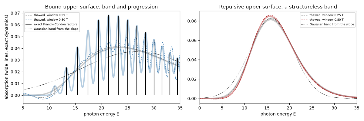
small-oscillation period on the upper surface T = 2.810, level spacing 2 pi hbar / T = 2.236 at the bottom of the well
exact level spacing at the band centre: 1.674
Morse    , window 0.25 T: correlation of exact and thawed spectra 0.999
Morse    , window 0.80 T: correlation of exact and thawed spectra 0.850
repulsive, window 0.25 T: correlation of exact and thawed spectra 1.000
repulsive, window 0.80 T: correlation of exact and thawed spectra 1.000

Check

Short-time dynamics fix the band (the thawed Gaussian is exact there); resolving the Morse progression needs longer times, where the thawed Gaussian misses the anharmonicity; on the repulsive surface it stays exact.

corr = {
    (name, frac): np.corrcoef(spectrum(E, times, C_ex, frac * T_vib), spectrum(E, times, C_tg, frac * T_vib))[0, 1]
    for name, C_ex, C_tg in [("Morse", C_morse_ex, C_morse_tg), ("repulsive", C_rep_ex, C_rep_tg)]
    for frac in (0.25, 0.8)
}
assert corr["Morse", 0.25] > 0.99 and corr["repulsive", 0.25] > 0.99 and corr["repulsive", 0.8] > 0.99
assert corr["Morse", 0.8] < 0.95
assert abs(T_vib - 2 * np.pi / (a_m * np.sqrt(2 * D_e))) < 1e-12
assert res.energies[i_c + 1] - res.energies[i_c] < 2 * np.pi / T_vib