Landau mean-field theory: order parameters from symmetry alone

Rather than derive a phase transition from a microscopic Hamiltonian, Landau (1937) asked what the free energy must look like near a continuous transition, given only the symmetry of an order parameter \(m\) that the disordered phase forbids from appearing at odd powers:

\[F(m, T) = a(T - T_C)\, m^2 + b\, m^4 - h\, m, \qquad a, b > 0.\]

Minimizing this quartic reproduces, from analyticity and symmetry alone, the qualitative shape of a continuous transition: one minimum at \(m=0\) above \(T_C\), a spontaneously broken pair of minima below it, and a susceptibility diverging on both sides. This example sits conceptually between Ising’s 1925 model and Onsager’s 1944 exact solution: Landau theory gets the qualitative picture of symmetry breaking right with no microscopic input at all, but its quantitative mean-field exponents (\(\beta = 1/2\), \(\gamma = 1\)) are simply wrong in two dimensions – Onsager’s exact solution gives \(\beta = 1/8\) instead – a discrepancy that the renormalization group would not fully explain for another three decades.

import matplotlib.pyplot as plt
import numpy as np

from physicskit.statphys.utils.landau_theory import (
    landau_equilibrium_magnetization,
    landau_free_energy,
    landau_susceptibility,
)

Tc = 2.0

The free-energy landscape above, at, and below T_C

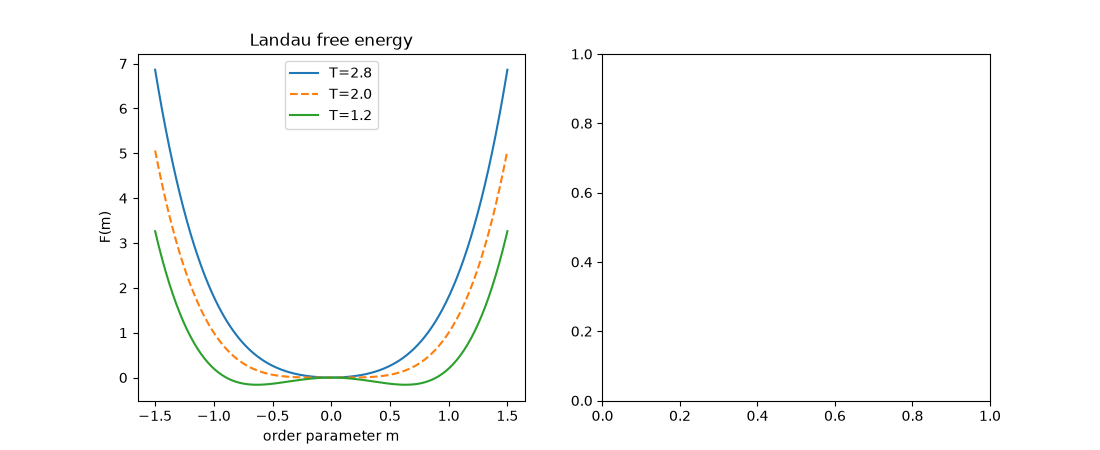
A single minimum at m=0 flattens at T_C and splits into a symmetric double well below it – the direct, visual signature of spontaneous symmetry breaking.

m_grid = np.linspace(-1.5, 1.5, 300)
fig, axes = plt.subplots(1, 2, figsize=(11, 4.5))
for T, style in zip([Tc + 0.8, Tc, Tc - 0.8], ["-", "--", "-"]):
    F = landau_free_energy(m_grid, T=T, Tc=Tc)
    axes[0].plot(m_grid, F, style, label=f"T={T:.1f}")
axes[0].set_xlabel("order parameter m")
axes[0].set_ylabel("F(m)")
axes[0].set_title("Landau free energy")
axes[0].legend()

<matplotlib.legend.Legend object at 0x375e36780>

Equilibrium magnetization and the diverging susceptibility

The equilibrium m(T) follows the mean-field beta=1/2 power law below T_C, while chi(T) diverges symmetrically on both sides with the mean-field gamma=1 exponent (and the universal amplitude ratio of 2 between the two sides).

T_grid = np.linspace(0.2, 4.0, 400)
m_eq = landau_equilibrium_magnetization(T_grid, Tc=Tc)
chi = landau_susceptibility(T_grid, Tc=Tc)

ax2 = axes[1]
ax2.plot(T_grid, m_eq, color="tab:blue", label="m(T)")
ax2.set_xlabel("T")
ax2.set_ylabel("m(T)", color="tab:blue")
ax2.axvline(Tc, color="gray", linestyle=":")

ax2b = ax2.twinx()
ax2b.plot(T_grid, np.clip(chi, 0, 10), color="tab:red", label=r"$\chi(T)$")
ax2b.set_ylabel(r"$\chi(T)$ (clipped)", color="tab:red")
ax2.set_title("Order parameter and susceptibility")

plt.tight_layout()

print(f"m(T_C - 0.8) = {landau_equilibrium_magnetization(Tc - 0.8, Tc):.4f}")
print(f"m(T_C + 0.8) = {landau_equilibrium_magnetization(Tc + 0.8, Tc):.4f}")

m(T_C - 0.8) = 0.6325
m(T_C + 0.8) = 0.0000

Field response: a symmetry-breaking jump below T_C, none above it

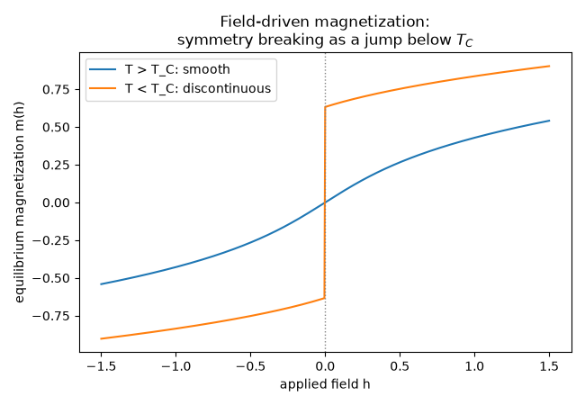
Everything above used the zero-field free energy. Turning on the linear field term h tilts the double well and lets the global equilibrium magnetization be traced as h is swept, at fixed T, using the same minimizer with its h argument now nonzero. Above T_C, where there is only ever one minimum, m(h) responds smoothly and continuously through h=0. Below T_C, the field tips the balance between the two (otherwise degenerate) symmetry-broken minima, so the globally stable branch jumps discontinuously from the negative to the positive minimum right at h=0 – a mean-field, equilibrium-tracking cartoon of the discontinuous jump a real ferromagnet’s magnetization undergoes as an applied field reverses sign below its own Curie point.

h_grid = np.linspace(-1.5, 1.5, 601)
fig, ax = plt.subplots(figsize=(6.5, 4.5))
for T, label in zip([Tc + 0.8, Tc - 0.8], ["T > T_C: smooth", "T < T_C: discontinuous"]):
    m_of_h = np.array([landau_equilibrium_magnetization(T, Tc, h=h) for h in h_grid])
    ax.plot(h_grid, m_of_h, label=label)
ax.axvline(0.0, color="gray", linestyle=":", linewidth=1)
ax.set_xlabel("applied field h")
ax.set_ylabel("equilibrium magnetization m(h)")
ax.set_title("Field-driven magnetization:\nsymmetry breaking as a jump below $T_C$")
ax.legend()
plt.tight_layout()
plt.show()